2 Foundations: the saddle-point toolkit

2.1 The sum versus its largest term

The previous lecture ended at a wall. We derived the Boltzmann distribution from maximum entropy, identified the softmax as a partition function over labels, and then saw the same object become intractable: for \(N\) binary units, \(Z = \sum_x e^{-\beta E(x)}\) has \(2^N\) terms, and already at \(N = 300\) that is \(\sim 2 \times 10^{90}\) — ten orders of magnitude more terms than there are atoms in the observable universe (Section 1.6). We left the number on the board as a provocation.

And yet physicists have computed with \(Z\) — phase diagrams, heat capacities, critical temperatures — for a century and a half. The question, then: if we can never sum it, how does anyone ever compute anything with \(Z\)?

The resolution is not cleverness about the sum; it is a change of target. We give up on \(Z\) itself and compute its logarithmic density, \(\frac{1}{N} \log Z\), in the limit where physics and machine learning both live — \(N\) large: \(10^{23}\) atoms, \(10^6\) pixels, \(10^9\) weights. In that limit a simplification takes over: when the exponent of a sum is extensive — proportional to \(N\) — the sum is dominated by its largest term, and \(\frac{1}{N} \log Z\) can be read off from that single term alone. The central dichotomy — for this lecture and for the course — is the sum versus its largest term: the sum is hopeless, the largest term is a one-dimensional maximization.

The technology that makes this precise is Laplace’s method, known to physicists as the saddle-point approximation, and it is built out of one integral — the Gaussian. The chain runs: Gaussian integral, then Laplace’s method on top of it, then Stirling’s formula as its canonical corollary, and finally the free energy as a saddle — mean-field theory in embryo and the seed of all of Module 2. Before the new machinery, we spend a few compressed pages placing \(Z\) properly: on the ladder of ensembles, and as a generating function — the corollaries the previous lecture deferred.

Everything below is stated for sums or for integrals as convenient. A sum over configurations and an integral over configurations differ by a measure that contributes nothing at the exponential order we work in, so \(\sum_x \leftrightarrow \int \mathrm{d}x\) throughout; we lead discrete this week, per the course convention, and switch to continuous from Module 3 on.

2.2 The ensemble ladder, in one panel

In the previous lecture, the canonical distribution arrived by inference: maximum entropy under a mean-energy constraint. The physics tradition arrives at the same object through a different door — as one rung on a ladder of ensembles, the systematization owed to Gibbs (1902) — and we spend one compressed panel placing the course on that ladder, because the choice of rung is a choice of what is held fixed. This is master’s material; we state it and move on.

Ensemble	Held fixed	Distribution	Thermodynamic potential
microcanonical	\(E,\ N\)	\(p(x) = 1/\Omega(E)\) (uniform on the shell)	\(S(E) = \log \Omega(E)\)
canonical	\(T,\ N\)	\(p(x) = e^{-\beta E(x)}/Z\)	\(F(T) = -T \log Z\)
grand-canonical	\(T,\ \mu\)	\(p(x) \propto e^{-\beta[E(x) - \mu N(x)]}\)	\(\Omega_G(T, \mu) = -T \log Z_G\)

The microcanonical rung is the previous lecture’s tombstone relation \(S = \log W\) dressed as an ensemble: fix the energy exactly, count the microstates, take the log. It is the only rung with no free dial — every other ensemble is reached from it by a Legendre transform, trading a conserved quantity for its conjugate field: \(E \leftrightarrow \beta\) takes microcanonical to canonical, \(N \leftrightarrow \mu\) takes canonical to grand-canonical, and the potentials in the last column are the transform partners. The general algebra is standard and we do not reproduce it (Schwarz 2023) — with one exception, because the course lives on the rung it lands on.

One rung, derived: the heat bath. The physics tradition’s route to the canonical distribution — the counterpart of the previous lecture’s inference route — is a three-line marginalization, and it is worth having both doors on record (Welling, Lu, and Holdijk 2026, sec. 3.2). Embed the system of interest in a much larger bath with which it exchanges energy, and let the pair be isolated at total energy \(E_\text{tot}\). The combined system sits on the microcanonical rung — uniform on its shell — and the system’s own distribution follows by tracing the bath out: when the system holds configuration \(x\), the bath is left with energy \(E_\text{tot} - E(x)\), and the probability of \(x\) is proportional to the number of ways the bath can accommodate that,

\[ p(x) \;\propto\; \Omega_\text{bath}\big(E_\text{tot} - E(x)\big) \;=\; \exp\!\Big[ S_\text{bath}\big(E_\text{tot} - E(x)\big) \Big], \]

using the first rung’s own relation \(S = \log \Omega\). Now use that the bath is large, \(E(x) \ll E_\text{tot}\), and expand its entropy — not its microstate count — to first order:

\[ S_\text{bath}\big(E_\text{tot} - E(x)\big) \;=\; S_\text{bath}(E_\text{tot}) \;-\; E(x)\, \underbrace{\frac{\partial S_\text{bath}}{\partial E}}_{\;\equiv\; 1/T} \;+\; \mathcal{O}\big(E(x)^2\, \partial_E^2 S_\text{bath}\big), \]

the canonical rung, from the microcanonical one

where \(1/T \equiv \partial S / \partial E\) is the microcanonical definition of temperature — the slope of the bath’s entropy against energy, the one dial the bath presents to anything coupled to it. The leading term is independent of \(x\) and absorbs into the normalization, and what remains is \(p(x) = e^{-E(x)/T} / Z\): the canonical rung, derived rather than listed. The reading to keep: the Boltzmann factor counts bath microstates — a configuration is penalized by exactly the entropy the bath must surrender to fund its energy, \(e^{-\Delta S_\text{bath}}\). The dropped curvature term is where the assumption of a much larger bath enters quantitatively: \(\partial_E^2 S_\text{bath} = -1/(T^2 C_\text{bath})\) vanishes as the bath’s heat capacity grows, which is the precise content of “the bath’s temperature is unaffected by the exchange.” And the two doors now visibly open onto one room: The previous lecture manufactured \(\beta\) as the Lagrange multiplier of a mean-energy constraint; here the same \(\beta\) arrives as a physical slope, the bath’s entropy price per unit of energy. That the multiplier is the slope is the Legendre duality of the ladder, met in its most concrete instance.

What matters for us is where this course lives: on the canonical rung, almost without exception, from here to Module 5. The canonical ensemble is the natural home of learning problems — a model at fixed “temperature” (noise level, regularization strength) rather than fixed energy — and its potential \(F = -T \log Z\) is the object every module manipulates. The grand-canonical rung is listed for completeness; it will not reappear unless particle-number-like quantities do. (A symbol warning: the grand potential \(\Omega_G\) shares its letter with the microstate count \(\Omega(E)\) one row above — unrelated objects, distinguished by the subscript, and we will need only the latter.)

Trap

Ensemble equivalence — the statement that all rungs give the same physics — holds for mean values in the thermodynamic limit, but it fails for fluctuations and at phase transitions. The moment Module 2 studies broken symmetry, the distinction starts to matter.

2.3 The partition function as a generating function

Last time we noted that \(Z\) is “not a bookkeeping constant.” Differentiate \(\log Z(\beta)\) with respect to \(\beta\):

\[ \frac{\partial \log Z}{\partial \beta} = \frac{1}{Z} \sum_x (-E(x))\, e^{-\beta E(x)} = -\sum_x E(x)\, \underbrace{\frac{e^{-\beta E(x)}}{Z}}_{=\ p(x)} = -\langle E \rangle, \]

so that

\[ \langle E \rangle = -\frac{\partial \log Z}{\partial \beta} \]

mean energy from \(\log Z\)

⇒ Differentiating the log-partition function produces the observables — no additional summation over configurations required.

Differentiating again, the same product rule that produced \(-\langle E \rangle\) now produces both \(\langle E^2 \rangle\) and \(\langle E \rangle^2\):

\[ \frac{\partial^2 \log Z}{\partial \beta^2} = \langle E^2 \rangle - \langle E \rangle^2 = \operatorname{Var}(E) \;\geq\; 0, \]

and since \(\partial/\partial T = -\beta^2\, \partial/\partial \beta\), the heat capacity follows immediately:

\[ C \;=\; \frac{\partial \langle E \rangle}{\partial T} \;=\; \beta^2 \operatorname{Var}(E). \]

The pattern has a name: \(\log Z\) is a cumulant generating function — its \(\beta\)-derivatives are the cumulants of the energy — and the second identity says that a fluctuation (the energy variance, a property of the equilibrium ensemble sitting still) equals a response (the heat capacity, how the system reacts when you turn the temperature dial). This fluctuation–response pattern is not a curiosity of the energy: it is the seed of the susceptibility and fluctuation–dissipation results of Module 2, and of the information-theoretic identities of Module 5. As a bonus, \(\operatorname{Var}(E) \geq 0\) says \(\log Z\) is convex in \(\beta\) — a fact the Legendre transforms of the previous section quietly rely on.

The free energy ties the two derivatives together: \(F = -T \log Z = \langle E \rangle - TS\), the previous lecture’s identity, now backed by explicit derivatives. \(F\) is the object the next two sections learn to compute — and the object the variational methods of Module 2 learn to bound, via \(D_\mathrm{KL} \geq 0\).

Take-home 1

\(Z\) is a generating function: \(\langle E \rangle = -\partial \log Z / \partial \beta\) and \(\operatorname{Var}(E) = \partial^2 \log Z / \partial \beta^2\), so a fluctuation (energy variance) equals a response (heat capacity), \(C = \beta^2 \operatorname{Var}(E)\). Derivatives of \(\log Z\) are physics — which is why we always want \(\log Z\), never \(Z\).

Trap

\(\langle E \rangle = -\partial \log Z / \partial \beta\) holds at fixed couplings: the derivative moves \(\beta\) and nothing else. If the energy itself depends on \(\beta\) (or on \(T\), as effective Hamiltonians often do), differentiating silently adds terms. State what is held fixed before differentiating — always.

2.4 The engine: Gaussian integral, Laplace’s method, Stirling’s formula

The derivation builds the engine the rest of the course runs on. The problem is the dichotomy of the opening section: we cannot sum \(2^N\) terms, but we can find the largest one, and we need to know how good “keep only the largest term” is. Laplace’s method answers that question quantitatively, and the Gaussian integral is the piece that makes the answer computable.

The Gaussian integral. We start with the atom, the recurring integral of the course:

\[ I(a) = \int_{-\infty}^{\infty} \mathrm{d}x\; e^{-a x^2 / 2}, \qquad a > 0. \]

The integrand has no elementary antiderivative; the classic trick — which we carry out once in full and then invoke freely — is to compute the square of the integral and pass to polar coordinates, where the measure \(r\, \mathrm{d}r\) supplies exactly the missing factor:

\[ \begin{aligned} I^2(a) &= \int_{-\infty}^{\infty} \! \mathrm{d}x \int_{-\infty}^{\infty} \! \mathrm{d}y\; e^{-a (x^2 + y^2)/2} \\[4pt] &= \int_0^{2\pi} \! \mathrm{d}\varphi \int_0^{\infty} \! r\, \mathrm{d}r\; e^{-a r^2 / 2} = 2\pi \left[ -\frac{e^{-a r^2/2}}{a} \right]_0^{\infty} = \frac{2\pi}{a}, \end{aligned} \]

and therefore

\[ \int_{-\infty}^{\infty} \mathrm{d}x\; e^{-a x^2/2} = \sqrt{\frac{2\pi}{a}} \tag{2.1}\]

Gaussian integral

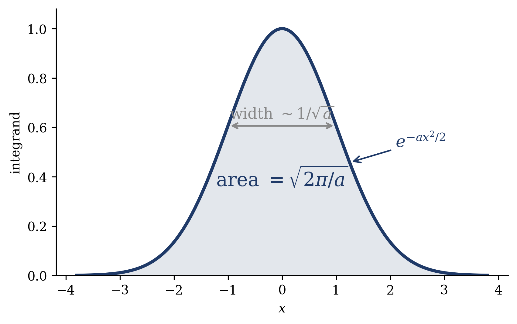
Figure 2.1 draws the statement: a bell curve of width \(\sim 1/\sqrt{a}\) enclosing an area \(\sqrt{2\pi/a}\) — sharper curvature, narrower peak, smaller area. For later use we state, result-first, the multivariate extension with a linear term (proved by completing the square and diagonalizing):

\[ \int \mathrm{d}^n x\; e^{-\frac{1}{2} x^\top \! A\, x + b^\top \! x} = \sqrt{\frac{(2\pi)^n}{\det A}}\; e^{\frac{1}{2} b^\top \! A^{-1} b}, \qquad A \succ 0. \]

Every Gaussian you will ever integrate in this course is Equation 2.1 plus a change of variables. This one labeled result already covers ① the Hubbard–Stratonovich transformation of Module 2, ② the Laplace approximation behind variational autoencoders, also Module 2, and ③ the transition kernel of every single step of a diffusion model, Module 4.

Show code

fig, ax = plt.subplots(figsize=(6.4, 3.8))
x = np.linspace(-3.8, 3.8, 400)
y = np.exp(-x**2 / 2)                          # a = 1
ax.fill_between(x, y, color=NAVY, alpha=0.12)
ax.plot(x, y, color=NAVY, lw=2.5)
y0 = np.exp(-0.5)
ax.annotate("", xy=(-1, y0), xytext=(1, y0),
            arrowprops=dict(arrowstyle="<->", color=GRAY, lw=1.4))
ax.text(0, y0 + 0.03, r"width $\sim 1/\sqrt{a}$", color=GRAY, ha="center", fontsize=12)
ax.text(0, 0.36, r"area $=\sqrt{2\pi/a}$", color=NAVY, ha="center", fontsize=15)
ax.annotate(r"$e^{-ax^2/2}$", xy=(1.25, np.exp(-1.25**2 / 2)), xytext=(2.1, 0.52),
            color=NAVY, fontsize=13, arrowprops=dict(arrowstyle="->", color=NAVY, lw=1.2))
ax.set_xlabel(r"$x$"); ax.set_ylabel("integrand")
ax.set_ylim(0, 1.08)
plt.show()

Figure 2.1: The atom of the course: the Gaussian integrand \(e^{-ax^2/2}\) (drawn for \(a=1\)) encloses an area of exactly \(\sqrt{2\pi/a}\), with characteristic width \(1/\sqrt{a}\) — sharper curvature \(a\) means a narrower, smaller-area peak. Every Gaussian integral from here to Module 4 — Hubbard–Stratonovich, the VAE’s Laplace approximation, each diffusion kernel — is this one integral after a change of variables.

Laplace’s method. The picture comes first, because the picture is the method. Consider an integral of the form

\[ I_N = \int \mathrm{d}x\; e^{N f(x)}, \]

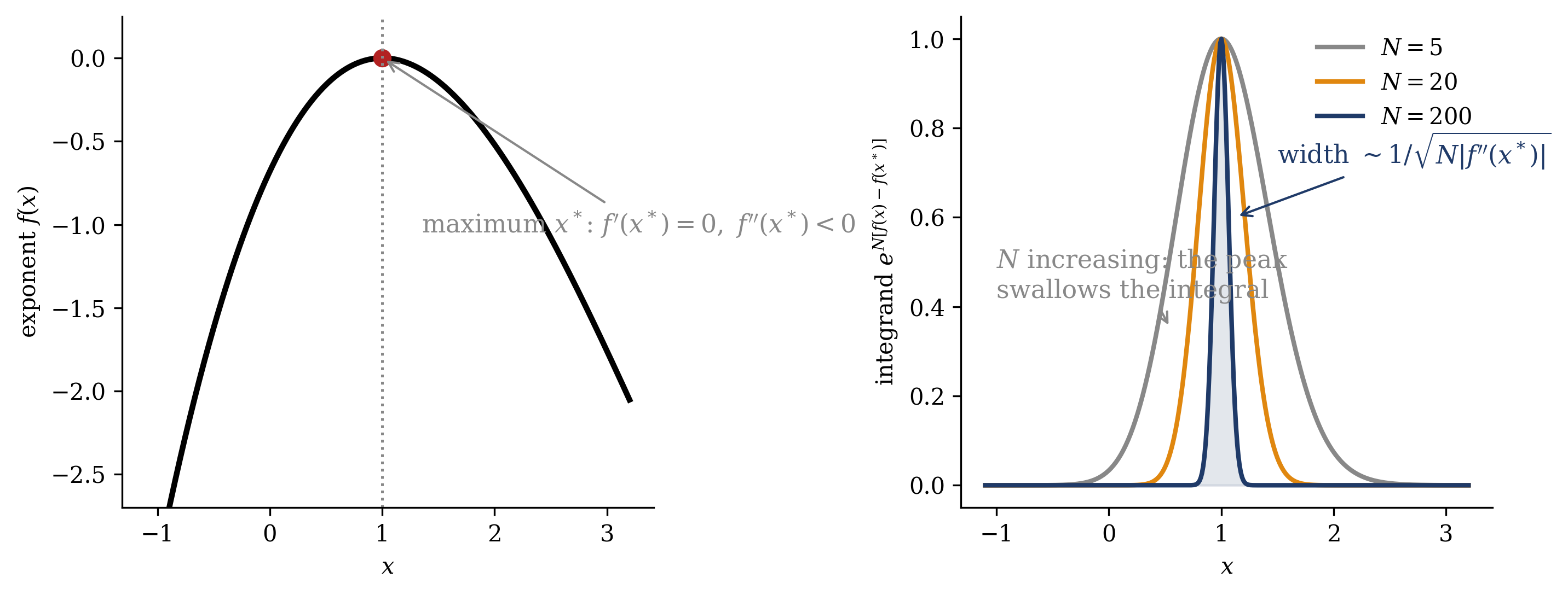
where \(N\) is large and the exponent is extensive — the factor \(N\) multiplies a smooth, \(N\)-independent function \(f(x)\) with ① a unique interior maximum at \(x^*\), so \(f'(x^*) = 0\) and \(f''(x^*) < 0\). (A warning on symbols: \(f(x)\) here is a generic exponent, not the free-energy density \(f(m)\) of the next section — the clash is standard in the literature, and we flag it rather than pretend it away.) Figure 2.2 shows what the factor \(N\) does to the integrand: \(e^{N f(x)}\) is the function \(e^{f(x)}\) raised to the \(N\)-th power, so every ratio between the peak and the rest gets amplified \(N\)-fold in the exponent, and the integrand collapses onto a shrinking neighborhood of \(x^*\). The integral is a sum of contributions; as \(N\) grows, one contribution swallows all the others.

Show code

f = lambda x: -0.6 * (x - 1)**2 + 0.08 * (x - 1)**3   # smooth, unique max at x*=1, f*=0
xs = 1.0                                              # x*, with f''(x*) = -1.2
fig, (a1, a2) = plt.subplots(1, 2, figsize=(9.6, 3.7))
xx = np.linspace(-1.1, 3.2, 400)
a1.plot(xx, f(xx), color="k", lw=2.5)
a1.plot([xs], [0], "o", color=RED, ms=7)
a1.axvline(xs, color=GRAY, ls=":", lw=1.2)
a1.annotate(r"maximum $x^*$: $f'(x^*)=0,\ f''(x^*)<0$", xy=(xs, 0),
            xytext=(1.35, -1.05), color=GRAY, fontsize=11, ha="left",
            arrowprops=dict(arrowstyle="->", color=GRAY, lw=1))
a1.set_xlabel(r"$x$"); a1.set_ylabel(r"exponent $f(x)$"); a1.set_ylim(-2.7, 0.25)
for N, c in [(5, GRAY), (20, ORANGE), (200, NAVY)]:
    g = np.exp(N * f(xx))
    a2.plot(xx, g, color=c, lw=2, label=f"$N={N}$")
    if N == 200:
        a2.fill_between(xx, g, color=NAVY, alpha=0.12)
a2.annotate("$N$ increasing: the peak\nswallows the integral", xy=(0.55, 0.35),
            xytext=(-1.0, 0.42), color=GRAY, fontsize=11,
            arrowprops=dict(arrowstyle="->", color=GRAY, lw=1))
a2.annotate(r"width $\sim 1/\sqrt{N|f''(x^*)|}$", xy=(1.12, 0.6), xytext=(1.5, 0.72),
            color=NAVY, fontsize=11, arrowprops=dict(arrowstyle="->", color=NAVY, lw=1))
a2.set_xlabel(r"$x$"); a2.set_ylabel(r"integrand $e^{N[f(x)-f(x^\ast)]}$")
a2.legend(frameon=False, fontsize=10, loc="upper right")
fig.tight_layout(); plt.show()

Figure 2.2: The central picture of the lecture. Left: a smooth exponent \(f(x)\) with a unique maximum at \(x^*\), where \(f'(x^*) = 0\) and \(f''(x^*) < 0\). Right: the integrand \(e^{N[f(x) - f(x^*)]}\) for \(N = 5\), \(20\), and \(200\) — each increase in \(N\) sharpens the peak, whose width shrinks as \(1/\sqrt{N |f''(x^*)|}\), until the neighborhood of \(x^*\) carries essentially the entire integral. Laplace’s method is the statement that this peak swallows the whole integral as \(N \to \infty\).

The calculation formalizes the picture in three moves. Taylor-expand the exponent about \(x^*\) — about the maximum, precisely because the linear term vanishes there and the quadratic term is the leading survivor:

\[ f(x) = f(x^*) + \tfrac{1}{2} f''(x^*)\, (x - x^*)^2 + \mathcal{O}\!\left((x - x^*)^3\right). \]

Substitute, pull the constant out of the integral, and recognize what remains:

\[ I_N \;\approx\; e^{N f(x^*)} \int \mathrm{d}x\; e^{-\frac{1}{2} N |f''(x^*)|\, (x - x^*)^2}, \]

which is Equation 2.1 with curvature \(a = N |f''(x^*)|\). Hence

\[ \boxed{\; I_N = \int \mathrm{d}x\; e^{N f(x)} \;\approx\; e^{N f(x^*)} \sqrt{\frac{2\pi}{N\, |f''(x^*)|}} \;} \tag{2.2}\]

Laplace’s method

Taking the logarithm and dividing by \(N\) gives the form we will actually use, over and over:

\[ \frac{1}{N} \log I_N = f(x^*) + \mathcal{O}\!\left(\frac{\log N}{N}\right) \;\longrightarrow\; f(x^*) \quad (N \to \infty). \]

⇒ To leading order in \(N\), an integral — or a sum — with an extensive exponent equals its single largest contribution; the Gaussian fluctuations around it are a \(1/\sqrt{N}\) correction that survives only in the subleading \(\log\) term. The \(2^N\) wall is not climbed; it is bypassed.

A remark on names, for recognition rather than use. The same idea for complex or oscillatory exponents — deform the integration contour through the point where \(f'(z) = 0\), a saddle point of the complex landscape — is the method of steepest descent, associated with Riemann and worked out by Debye (1909). Physicists say “saddle point” even in the real case, and so will we; when the replica literature of Module 2 says it, this is what it means. We will only ever need the real, Laplace version (MacKay 2003; Sethna 2021).

Stirling’s formula. The engine’s canonical corollary is Stirling’s formula — published in 1730, a century before Laplace’s method made it a one-liner — and it is the bridge back to the previous lecture’s entropy counting. Start from the Gamma-function representation of the factorial and bring it to the Laplace template by substituting \(x = n y\):

\[ n! = \int_0^{\infty} \mathrm{d}x\; x^n e^{-x} \;\overset{x = ny}{=}\; n^{\,n+1} \int_0^{\infty} \mathrm{d}y\; e^{\,n (\log y \,-\, y)}. \]

The exponent \(f(y) = \log y - y\) has its maximum at \(f'(y^*) = 1/y^* - 1 = 0\), i.e. \(y^* = 1\), with \(f(1) = -1\) and \(f''(1) = -1\). Applying Equation 2.2,

\[ n! \;\approx\; n^{\,n+1}\, e^{-n} \sqrt{\frac{2\pi}{n}} = \sqrt{2\pi n}\; \Big(\frac{n}{e}\Big)^{\!n}, \]

or in the logarithmic form we will use:

\[ \log n! = n \log n - n + \tfrac{1}{2} \log(2\pi n) + \mathcal{O}(1/n) \tag{2.3}\]

Stirling’s formula

⇒ Stirling is Laplace applied to a factorial — and it is precisely the tool that turns the previous lecture’s entropy counting \(S = \log W\), with \(W\) a product of factorials, into a smooth, differentiable entropy density that calculus can grip. That conversion — counting into calculus — is what the next section puts to work.

Trap

The saddle point is a large-\(N\) statement — exact only as \(N \to \infty\), and only when the exponent is extensive (\(\propto N\)). At finite \(N\) the Gaussian prefactor \(\sqrt{2\pi / N|f''(x^*)|}\) is a real, quantitative correction, not decoration (the worked example below puts numbers on it). Writing \(\int e^{Nf} \approx e^{N f(x^*)}\) with no conditions attached is a frequent abuse in the literature — attach the regime, every time.

Take-home 2

Laplace’s method: \(\frac{1}{N} \log \int \mathrm{d}x\; e^{N f(x)} \to f(x^*)\), where \(x^*\) maximizes \(f\). In the large-\(N\) limit a sum or integral equals its largest term; the width of the peak around it is \(\sim 1/\sqrt{N}\), and the Gaussian integral \(\sqrt{2\pi/a}\) computes the correction. This is the universal computational strategy of the course.

2.5 The free energy as a saddle

Applying the engine to \(Z\) itself yields mean-field theory — the preview of Module 2.

The move that makes a \(2^N\)-term sum tractable is a reorganization. Take \(N\) binary spins \(x_i = \pm 1\) and define the order parameter \(m = \frac{1}{N} \sum_i x_i\), the magnetization — one number summarizing a configuration. Instead of summing over configurations one by one, group them by their value of \(m\). Two facts make the grouped sum exponential in form. First, the number of configurations with magnetization \(m\) is a binomial coefficient, \(\binom{N}{N(1+m)/2}\), and Stirling’s formula — this is exactly where Equation 2.3 does its work — turns it into \(e^{N s(m)}\) with the entropy density

\[ s(m) = \log 2 - \tfrac{1}{2}\left[ (1+m) \log (1+m) + (1-m) \log(1-m) \right]. \]

Second, when the energy depends on the configuration only through \(m\) — true for all-to-all (mean-field) couplings, e.g. \(E = -\frac{J}{2N} \big(\sum_i x_i\big)^2 = N \varepsilon(m)\) with \(\varepsilon(m) = -\frac{J}{2} m^2\) — each grouped term carries the weight \(e^{-\beta N \varepsilon(m)}\). The partition function collapses to a sum over the \(N+1\) values of \(m\):

\[ Z = \sum_m e^{N \left[ s(m) - \beta\, \varepsilon(m) \right]}. \]

This is precisely the Laplace template — an extensive exponent, a sum we may read as an integral — so Equation 2.2 applies verbatim, and the free-energy density \(f = F/N\) becomes

\[ \boxed{\; f \;=\; -\frac{1}{\beta N} \log Z \;\longrightarrow\; \min_m \left[\, \varepsilon(m) - T\, s(m) \,\right] \quad (N \to \infty) \;} \tag{2.4}\]

free-energy density as a saddle

⇒ The free energy is the minimum, over the order parameter, of “energy minus temperature times entropy”: a \(2^N\)-term sum has collapsed to a one-dimensional minimization, and the minimizer \(m^*\) is the equilibrium value of the order parameter. (The maximum of \(s - \beta \varepsilon\) becomes a minimum of \(\varepsilon - Ts\) under the overall minus sign — hence “minimize the free energy,” the phrasing every physics course drills.) Note the symbols doing double duty, as flagged above: \(f(m)\) is now a free-energy density and \(s(m)\) an entropy density — lowercase for per-spin quantities, reserving \(F\) and \(S\) for totals.

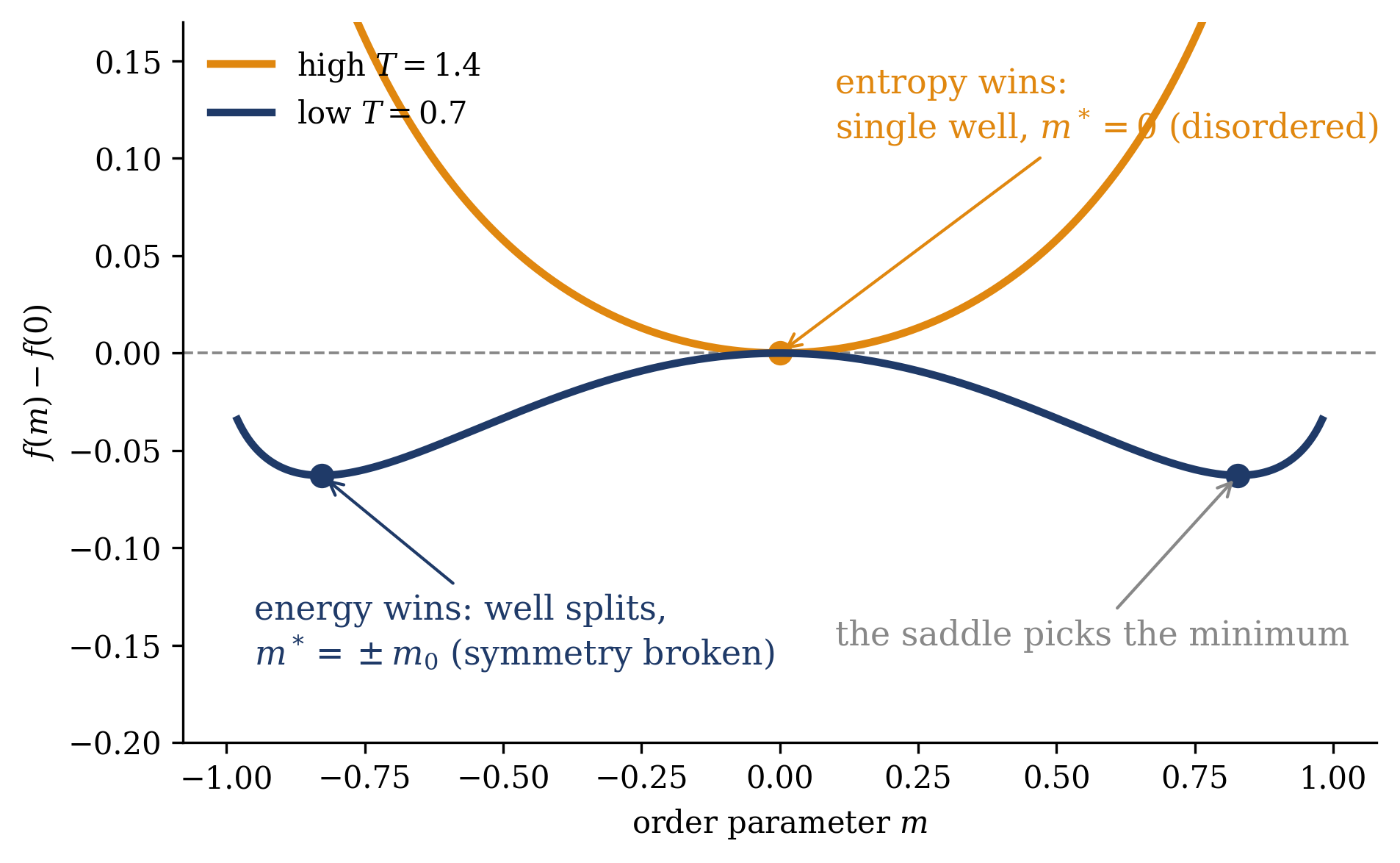
Everything thermodynamically interesting now lives in the shape of \(f(m) = \varepsilon(m) - T s(m)\), and the temperature is the dial that deforms it. Figure 2.3 draws the competition for the mean-field energy above. At high \(T\) the entropy term dominates: \(f(m)\) has a single well at \(m^* = 0\), the disordered state — maximal entropy, no net magnetization. At low \(T\) the energy term wins: the single well splits into two symmetric wells at \(m^* = \pm m_0\), and the system must settle into one of them. That splitting is spontaneous symmetry breaking, and the calculation we just sketched — group by an order parameter, Stirling the count, saddle the sum — is mean-field theory. We have done it here for the one energy where it is exact; doing it in full on the Hopfield network, and repairing it when it is not exact, is the business of Module 2 (Weeks 5–7).

Show code

def s(m):                                    # entropy density of N Ising spins
    m = np.clip(m, -0.999999, 0.999999)
    return np.log(2) - 0.5 * ((1 + m) * np.log(1 + m) + (1 - m) * np.log(1 - m))
eps = lambda m: -m**2 / 2                     # mean-field energy density, T_c = 1
m = np.linspace(-0.98, 0.98, 400)
fig, ax = plt.subplots(figsize=(6.6, 4.0))
ax.axhline(0, color=GRAY, ls="--", lw=0.9)
for T, c, lab in [(1.4, ORANGE, r"high $T=1.4$"), (0.7, NAVY, r"low $T=0.7$")]:
    fm0 = (eps(m) - T * s(m)) - (eps(0) - T * s(0))
    ax.plot(m, fm0, color=c, lw=2.5, label=lab)
    if T > 1:
        ax.plot([0], [0], "o", color=ORANGE, ms=7)
    else:                                     # mark the two symmetric minima
        i = np.argmin(fm0)
        ax.plot([m[i], -m[i]], [fm0[i], fm0[i]], "o", color=NAVY, ms=7)
        mstar, ystar = m[i], fm0[i]
ax.annotate("entropy wins:\nsingle well, $m^*=0$ (disordered)", xy=(0, 0),
            xytext=(0.1, 0.11), color=ORANGE, fontsize=11,
            arrowprops=dict(arrowstyle="->", color=ORANGE, lw=1))
ax.annotate("energy wins: well splits,\n$m^*=\\pm m_0$ (symmetry broken)", xy=(mstar, ystar),
            xytext=(-0.95, -0.16), color=NAVY, fontsize=11, ha="left",
            arrowprops=dict(arrowstyle="->", color=NAVY, lw=1))
ax.annotate("the saddle picks the minimum", xy=(-mstar, ystar), xytext=(0.1, -0.15),
            color=GRAY, fontsize=11, ha="left",
            arrowprops=dict(arrowstyle="->", color=GRAY, lw=1))
ax.set_xlabel(r"order parameter $m$"); ax.set_ylabel(r"$f(m)-f(0)$")
ax.set_ylim(-0.2, 0.17); ax.legend(frameon=False, fontsize=10, loc="upper left")
fig.tight_layout(); plt.show()

Figure 2.3: The free-energy saddle, drawn for the all-to-all ferromagnet \(\varepsilon(m) = -m^2/2\) (so \(T_c = 1\)), as \(f(m) - f(0)\) against the order parameter \(m\). At high temperature (\(T = 1.4\), orange) entropy dominates and the free energy has a single well at \(m^* = 0\): the disordered state. At low temperature (\(T = 0.7\), navy) energy dominates and the well splits into two symmetric minima at \(m^* = \pm m_0 \approx \pm 0.83\): the saddle must pick one — spontaneous symmetry breaking, and mean-field theory in embryo. Module 2 performs this calculation on real energies.

Take-home 3

The saddle-point method turns the free energy into a minimization: \(f = \min_m \left[ \varepsilon(m) - T s(m) \right]\) — the competition between energy and entropy resolved by one dominant order-parameter value. This is mean-field theory: planted here, solved properly in Module 2.

2.6 Example: how good is the largest term?

The approximation needs a reality check with actual numbers — first on Stirling, then on the concentration claim itself.

Stirling’s accuracy. Compare \(\log n!\) computed exactly against the leading form \(n \log n - n\) and against the corrected form that keeps the Gaussian prefactor, \(n \log n - n + \frac{1}{2} \log(2\pi n)\):

\(n\)	\(\log n!\) (exact)	\(n \log n - n\)	\(+\, \frac{1}{2}\log(2\pi n)\)	rel. err. (leading)	rel. err. (corrected)
\(2\)	\(0.693\)	\(-0.614\)	\(0.652\)	—	\(6 \times 10^{-2}\)
\(5\)	\(4.787\)	\(3.047\)	\(4.771\)	\(0.36\)	\(3 \times 10^{-3}\)
\(10\)	\(15.104\)	\(13.026\)	\(15.096\)	\(0.14\)	\(5 \times 10^{-4}\)
\(100\)	\(363.739\)	\(360.517\)	\(363.739\)	\(0.9\%\)	\(2 \times 10^{-6}\)

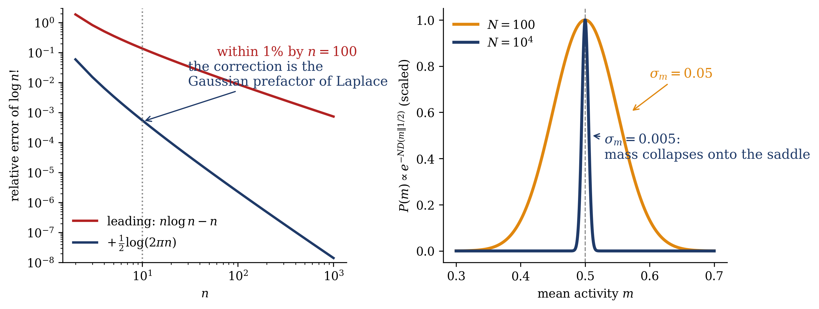
The left panel of Figure 2.4 plots the trend. Two readings. First, the leading form — the one we will routinely use — is within \(1\%\) by \(n = 100\) and improves steadily; for the \(n \sim 10^2\)–\(10^{23}\) of our applications it is quantitatively excellent. Second, and more instructive: the error of the leading form is the \(\frac{1}{2}\log(2\pi n)\) term — literally the Gaussian prefactor of Equation 2.2 — and restoring it nails the answer to \(5 \times 10^{-4}\) already at \(n = 10\). The correction we usually drop is not mysterious; it is the width of the peak, and we know its formula.

Binomial concentration — the \(2^N\) wall revisited. Now the concentration claim, on the simplest possible system: \(N\) unbiased binary units, every configuration equally likely. The fraction of configurations with mean activity \(m\) is governed by an exponential of the entropy deficit, \(P(m) \propto e^{-N D(m \| 1/2)}\) — in the language of large deviations, \(D(m\|1/2)\) is the rate function, here used informally — peaked at \(m = 1/2\) with standard deviation

\[ \sigma_m = \frac{1}{2\sqrt{N}}. \]

Put numbers on it: for \(N = 10^2\), \(10^4\), and \(10^6\), the width is \(\sigma_m = 0.05\), \(0.005\), and \(5 \times 10^{-4}\), respectively.

The right panel of Figure 2.4 draws the collapse. For \(N = 100\) the sum has \(2^{100} \approx 1.3 \times 10^{30}\) terms — already unsummable — yet the distribution over the order parameter is a bump of width \(0.05\); at \(N = 10^4\) it is a spike. All but a vanishing fraction of the \(2^N\) configurations are crowded into a sliver of width \(1/\sqrt{N}\) around the dominant value of \(m\) — which is exactly why keeping only the largest term is legitimate, and why its error is the Gaussian factor we computed rather than something unknown.

Show code

fig, (a1, a2) = plt.subplots(1, 2, figsize=(9.6, 3.7))
# left: accuracy of Stirling's formula against the exact log-factorial
n = np.arange(2, 1001)
exact = gammaln(n + 1)
lead = n * np.log(n) - n
corr = lead + 0.5 * np.log(2 * np.pi * n)
a1.loglog(n, np.abs(lead - exact) / exact, color=RED, lw=2, label=r"leading: $n\log n-n$")
a1.loglog(n, np.abs(corr - exact) / exact, color=NAVY, lw=2,
          label=r"$+\,\frac{1}{2}\log(2\pi n)$")
a1.axvline(10, color=GRAY, ls=":", lw=1.2)
a1.annotate(r"within 1% by $n=100$", xy=(100, 9e-3), xytext=(60, 8e-2),
            color=RED, fontsize=11)
a1.annotate("the correction is the\nGaussian prefactor of Laplace", xy=(10, 5e-4),
            xytext=(30, 8e-3), color=NAVY, fontsize=11,
            arrowprops=dict(arrowstyle="->", color=NAVY, lw=1))
a1.set_xlabel(r"$n$"); a1.set_ylabel(r"relative error of $\log n!$")
a1.set_ylim(1e-8, 3); a1.legend(frameon=False, fontsize=10, loc="lower left")
# right: binomial concentration of the mean activity onto m = 1/2
def Dkl(m):
    m = np.clip(m, 1e-12, 1 - 1e-12)
    return np.log(2) + m * np.log(m) + (1 - m) * np.log(1 - m)
mm = np.linspace(0.3, 0.7, 800)
a2.axvline(0.5, color=GRAY, ls="--", lw=0.9)
for N, c, lab in [(100, ORANGE, r"$N=100$"), (10000, NAVY, r"$N=10^4$")]:
    p = np.exp(-N * Dkl(mm)); p /= p.max()               # scaled to unit peak
    a2.plot(mm, p, color=c, lw=2.5, label=lab)
a2.annotate(r"$\sigma_m=0.05$", xy=(0.57, 0.6), xytext=(0.6, 0.75),
            color=ORANGE, fontsize=11, arrowprops=dict(arrowstyle="->", color=ORANGE, lw=1))
a2.annotate("$\\sigma_m=0.005$:\nmass collapses onto the saddle", xy=(0.508, 0.5),
            xytext=(0.53, 0.4), color=NAVY, fontsize=11,
            arrowprops=dict(arrowstyle="->", color=NAVY, lw=1))
a2.set_xlabel(r"mean activity $m$")
a2.set_ylabel(r"$P(m)\propto e^{-N D(m\|1/2)}$ (scaled)")
a2.legend(frameon=False, fontsize=10, loc="upper left")
fig.tight_layout(); plt.show()

Figure 2.4: Left: relative error of \(\log n!\) for the leading Stirling form \(n \log n - n\) (red) and the corrected form with the \(\frac{1}{2}\log(2\pi n)\) term (navy) — the leading form is within \(1\%\) by \(n = 100\), and the correction, which is precisely the Gaussian prefactor of Laplace’s method, is accurate to \(5 \times 10^{-4}\) already at \(n = 10\). Right: the distribution \(P(m) \propto e^{-N D(m \| 1/2)}\) of the mean activity of \(N\) unbiased binary units, for \(N = 100\) (\(\sigma_m = 0.05\), orange) and \(N = 10^4\) (\(\sigma_m = 0.005\), navy): the mass collapses as \(1/\sqrt{N}\) onto the saddle.

We never compute \(Z\); we compute \(\frac{1}{N} \log Z\) — and one term is enough. The \(2^N\) terms are all still there, but almost every one of them sits in a sliver of width \(1/\sqrt{N}\) around the saddle. Evaluating the saddle is \(\mathcal{O}(1)\); the other \(2^N - 1\) terms are a correction we compute analytically and never enumerate.

For the mean-field energy above there is a single saddle. For real energies — short-range, structured, disordered — the landscape \(f(m)\) grows many saddles, and deciding which ones to trust, and how to correct them, is the central question of Module 2: the TAP equations, belief propagation and message passing, and the replica method are three answers to that one question.

2.7 Loose ends and scope

Two loose ends from the previous lecture, then the scope of what this lecture skipped.

Maximum entropy, generalized. The previous lecture’s derivation used a single constraint — the mean energy — and produced a single multiplier, \(\beta\). The generalization is immediate and worth stating result-first: maximizing entropy subject to \(K\) constraints \(\langle f_k(x) \rangle = c_k\) yields the exponential family

\[ p(x) \;\propto\; \exp\!\Big( -\sum_{k=1}^{K} \lambda_k f_k(x) \Big), \]

one Lagrange multiplier per constraint, by the same variational calculation run in parallel (Jaynes 1957). Energy-based models, logistic regression, and Markov random fields are all the same object under different constraint sets — a unification Module 1 uses from Week 2 on. We do not re-run the derivation; the previous lecture’s single-constraint version plus “one multiplier per constraint” is the whole proof idea.

Scope. Three things this lecture deliberately did not do. We used the language of large deviations — rate function, concentration — informally, without the rigorous theory (Cramér, Varadhan); the informal version is all we need. We stayed with the real-variable Laplace method and never deformed a contour; the complex-analytic steepest descent is named so that you recognize it in the literature, not developed. And we asserted ensemble equivalence for mean values without proof, while flagging where it fails. Each of these has its rightful depth elsewhere; the corrections to the saddle point itself — the cases where the largest term is not enough — return as the spine of Module 2.

2.8 Outlook

Week 1 is complete, and its two lectures divide cleanly. Lecture 1 gave the object and the obstruction: probability from energy, \(p = e^{-\beta E}/Z\), and the \(2^N\) wall that makes \(Z\) intractable. Today gave the toolkit: \(\log Z\) as the generating function whose derivatives are physics, and the saddle-point chain — Gaussian integral, Laplace’s method, Stirling’s formula — that computes \(\frac{1}{N} \log Z\) asymptotically, collapsing the free energy onto a minimization over one order parameter. One idea, stated three ways: the largest term wins — in counting (Stirling), in integrals (Laplace), and in the free energy (the saddle).

Week 2 opens Module 1 with the Hopfield model: the Ising energy repurposed as an associative memory, and the first time in this course that \(E(x)\) is something we design rather than measure. Designed energies raise quantitative questions — how many patterns can a network of \(N\) neurons store? — and when Week 2 quotes the answer (\(\alpha_c \approx 0.138\), as promised in Lecture 1) and Module 2 equips you with its logic, it will rest on exactly the calculation you saw today: write the free energy, find the saddle. Figure 2.3 reappears throughout the course in progressively richer forms.

The practitioner’s summary: when you see \(e^{N \cdot (\text{something})}\), do not sum — find where the exponent is largest; and when you see a Gaussian, you can integrate it.