Core (~1 h).Ho, Jain, and Abbeel (2020) — §2–3, read this time as a derivation rather than a recipe: you have already trained this model, and today every line of its loss acquires a name from the last three weeks. Alongside it Sohl-Dickstein et al. (2015), §1–2 — the founding construction, which cites Jarzynski (1997) explicitly; its title, Deep Unsupervised Learning using Nonequilibrium Thermodynamics, is a one-line summary of this module.
Optional background.Song, Durkan, et al. (2021) — which reweighting of the denoising loss restores an honest likelihood bound; today’s engineering section states the result. Karras et al. (2022) — the modern audit of the design space (schedules, scalings, samplers) once the construction is understood. Welling, Lu, and Holdijk (2026) — the companion text’s variational-diffusion chapters treat exactly this material.
Prerequisite reminder. From Week 10: denoising score matching (Equation 19.4), the forward noising process (Equation 20.1), the reverse-time SDE (Equation 20.2), and the transport-not-equilibration principle of Chapter 20. From Week 11: the Crooks ratio (Equation 21.3), dissipation as a forward/reverse path divergence (Equation 21.5), the AIS identity (Equation 22.3), and the Jensen-gap accounting (Equation 22.4). From Module 2: the ELBO as a variational free energy (Equation 14.6) and the closed-form Gaussian KL (Equation 14.4). New content: the discrete forward chain and its two-anchor posterior, the path-space bound and its per-step decomposition, the \(\varepsilon\)-parameterization and its identity with the score, and the audit of DDPM’s engineering choices.
23.1 A loss you have already minimized
In Machine Learning and Physics you trained a denoising diffusion probabilistic model, and the loss you minimized was a mean-squared error on noise: draw a data point, corrupt it to a random level \(t\), and train a network \(\varepsilon_\theta\) to guess the noise that was added,
Nothing in that expression looks like statistical mechanics. There is no partition function and no free energy; it reads as a regression, and it was presented to you as one. \(L_\text{simple}\) is the terminal point of a derivation that runs through everything Module 4 has built: it is a nonequilibrium free-energy estimator in the precise sense of Week 11 — a Jensen-gap bound whose slack is the dissipation of a transport, with the reverse path measure now carrying the parameters — and each of its terms is Week 10’s denoising score matching at one noise level. Ho, Jain, and Abbeel (2020) wrote the recipe; Sohl-Dickstein et al. (2015) had built the construction five years earlier, directly from the fluctuation-theorem literature. Today we run the derivation forward, from the corruption chain to the regression, and keep a ledger of every step at which an engineering decision — a choice not forced by the mathematics — enters. There are four, catalogued in Section 23.5.
The required tools are all in hand — the forward process and its melting barriers (Section 20.2), the reverse-time SDE (Equation 20.2), denoising score matching (Equation 19.4), and the path-measure bookkeeping of Week 11’s two lectures. The new content is how they assemble into an industrial object, and the discrete-time bookkeeping that assembly requires.
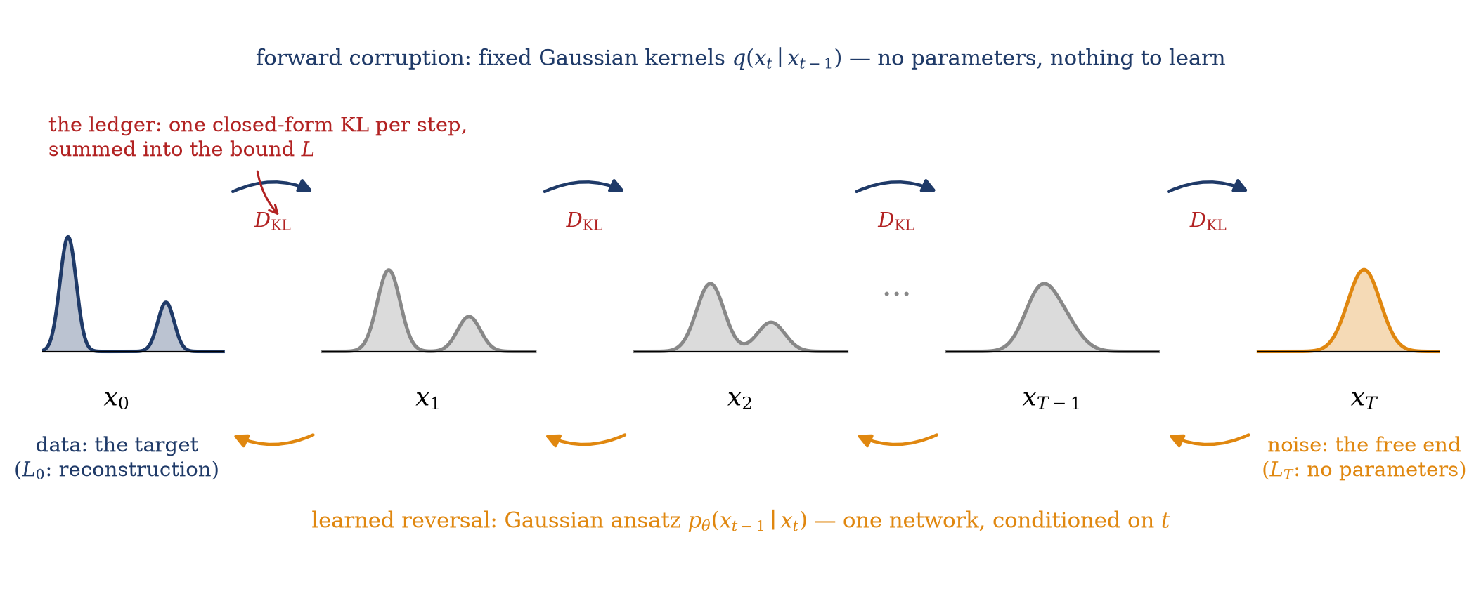
Figure 23.1: The central picture of the lecture — the DDPM as a double chain with a ledger. Top (navy): the forward corruption, a fixed Markov chain of Gaussian kernels \(q(x_t \mid x_{t-1})\) carrying the two-mode data density through blurred intermediates to a unit Gaussian; it contains no parameters and is never trained. Bottom (orange): the learned reversal, a Gaussian ansatz \(p_\theta(x_{t-1} \mid x_t)\) — one network, conditioned on \(t\) — run from noise back to data. Between the two chains sits the ledger: the variational bound decomposes into one closed-form Kullback–Leibler divergence per step, plus a parameter-free endpoint term \(L_T\) (does the corruption finish?) and a reconstruction term \(L_0\). Training a diffusion model is bookkeeping on this ledger.
23.2 The forward chain: the ladder, discretized
The DDPM forward process is Week 10’s corruption (Equation 20.1) written as a finite Markov chain. Fix a schedule\(\beta_1, \ldots, \beta_T \in (0, 1)\) and corrupt in \(T\) steps,
\[
q(x_t \mid x_{t-1}) \;=\; \mathcal{N}\!\big(x_t;\; \sqrt{1 - \beta_t}\; x_{t-1},\; \beta_t I\big),
\qquad t = 1, \ldots, T .
\]
A further notation warning: \(\beta_t\) here is a variance schedule — the fraction of variance replaced by fresh noise at step \(t\) — not an inverse temperature, exactly as the \(\beta_k\) of the AIS ladder (Section 22.3) was an annealing schedule. The field’s notation is entrenched and we keep it; no temperature appears anywhere today.
Write \(\alpha_t = 1 - \beta_t\) and \(\bar{\alpha}_t = \prod_{s=1}^t \alpha_s\). Composing the kernels collapses the chain into a single Gaussian: if \(x_{t-1} = \sqrt{\bar{\alpha}_{t-1}}\, x_0 + \sqrt{1 - \bar{\alpha}_{t-1}}\; \varepsilon'\), then one more step gives fresh noise of variance \(\alpha_t (1 - \bar{\alpha}_{t-1}) + \beta_t = 1 - \bar{\alpha}_t\), and by induction
the marginal: signal decays, total variance is preserved
The construction is variance-preserving — a unit-variance input stays at unit variance, \(\alpha_t + \beta_t = 1\) — and it is precisely the Ornstein–Uhlenbeck corruption of Equation 20.1 sampled at discrete times: setting \(\sqrt{\bar{\alpha}_t} = e^{-t_\text{phys}}\) reproduces Week 10’s transition law exactly, with \(\beta_t \approx 2\,\Delta t\) for small steps. Everything established there carries over unchanged — the endpoint is free (\(\bar{\alpha}_T \to 0\) makes \(x_T\) pure noise, whatever the data were), the intermediates are blurs whose barriers have melted (Figure 20.2), and the intermediates are exactly where denoising score matching trains.
The chain adds a closed form that the continuous picture did not need. Because the chain is Markov and every factor is Gaussian, the corruption step is exactly invertible when anchored at both ends: by Bayes,
the two-anchor posterior: the reversal, if you knew the answer
with — completing the square in \(x_{t-1}\), whose precision collects \(\alpha_t/\beta_t\) from the likelihood and \(1/(1 - \bar{\alpha}_{t-1})\) from the prior —
Equation 23.2 quantifies the challenge facing generation. Conditioned on where the trajectory started, one corruption step reverses in closed form — a Gaussian, with a mean that interpolates between the two anchors. But the starting point \(x_0\) is exactly what a generator does not have; it is the thing being generated. The model’s entire job will be to supply a substitute for the \(x_0\)-dependence of \(\tilde{\mu}_t\), and the substitute will turn out to be Week 10’s score.
23.3 The bound: dissipation acquires parameters
The generative model is the reverse chain of Figure 23.1: start at the free end and walk down,
with kernels to be specified in the next section. Its likelihood is a path integral, \(p_\theta(x_0) = \int \mathrm{d}x_{1:T}\, p_\theta(x_{0:T})\), and we evaluate it the way Week 11 evaluated every partition function: importance-sample the paths with the one path measure we can draw from — the forward corruption —
This display is Equation 22.3 with the roles reassigned: the forward corruption is the annealing protocol, the ratio is the AIS weight \(w\), and the quantity in the role of \(Z_K/Z_0\) is the model likelihood itself. In last week’s Lecture 1 dictionary \(\log w\) is a negative work, and Jensen’s inequality plays the part it played there (Equation 22.4): \(\log p_\theta(x_0) = \log \langle w \rangle \geq \langle \log w \rangle\), with the gap known exactly. Writing \(L(x_0; \theta) = -\langle \log w \rangle\) for the negative evidence lower bound and splitting \(p_\theta(x_{0:T}) = p_\theta(x_0)\, p_\theta(x_{1:T} \mid x_0)\),
the DDPM objective: a dissipation with parameters in the reverse measure
— the negative log-likelihood plus a Kullback–Leibler divergence between the forward path measure and the learned reverse one. The structure is Equation 21.5: the slack in the DDPM training objective is the dissipation of its own transport. In Week 11 the reverse path measure was fixed — the reversal of the forward kernels — and the dissipation was a cost to be accounted; here the reverse measure carries \(\theta\), and the dissipation is a cost to be minimized by gradient descent. Training pushes \(D_\mathrm{KL}(q_F \| p_\theta) \to 0\), that is, it drives the learned chain toward the exact time reversal of the corruption — and Anderson’s theorem (Equation 20.2) guarantees the target is reachable, since the exact reversal of a diffusion is again a diffusion, with Gaussian increments in the small-step limit. A model at zero dissipation is a reversible transport, and its bound is tight: \(L = -\log p_\theta(x_0)\).
Two remarks place the object among its relatives. First, in Week 7’s language Equation 23.3 is an ELBO (Equation 14.6): a diffusion model is a variational autoencoder whose latent variable is the entire path \(x_{1:T}\) and whose encoder is fixed — the corruption chain contains nothing to learn, which is why the encoder side contributes no gradients, and neither the reparameterization trick nor an amortization network appears anywhere. Second, the historical order ran the other way from the pedagogical one: Sohl-Dickstein et al. (2015) constructed exactly this bound by importing the Jarzynski–Crooks machinery into unsupervised learning, and Ho, Jain, and Abbeel (2020) made it competitive at scale five years later; the fluctuation-theorem lineage is a matter of citation record rather than a reinterpretation.
The bound as written is a single number per data point; training needs it as a sum of local terms. The move is the telescoping of Section 22.4, executed once more. For \(t \geq 2\), trade the forward kernel for the two-anchor posterior using Markovianity and Bayes (Equation 23.2),
and the marginal ratios telescope across the product \(\prod_{t=2}^{T}\), leaving \(q(x_T \mid x_0)\) at the far end — the same regrouping-by-configuration that proved Equation 21.3 and Equation 22.3. The bound falls apart into a ledger:
Each entry has a job. \(L_T\) contains no parameters at all: it measures whether the corruption finishes — whether \(q(x_T \mid x_0)\) has actually reached the unit Gaussian the reverse chain starts from — and with \(\bar{\alpha}_T \sim e^{-8}\) it is a fraction of a nat, fixed by the schedule. \(L_0\) is a reconstruction term for the final hop to data; for image models Ho, Jain, and Abbeel (2020) handle it with a discrete decoder over pixel bins, and we set it aside at a sentence. The sum in the middle is the substance: one Kullback–Leibler divergence per rung, between the two-anchor posterior — the reversal if you knew the answer — and the model’s kernel, which must manage without. Every distribution in sight is Gaussian, so every entry will be closed-form; no expectation in Equation 23.4 ever requires more than drawing \((x_0, \varepsilon, t)\) and evaluating a formula. The partition-function obstruction is absent: the model was built normalized, kernel by kernel.
Take-home 1
A DDPM is a fixed corruption chain plus a learned reverse chain, and its training objective Equation 23.3 is the negative log-likelihood plus the forward/reverse path divergence of Equation 21.5 — Week 11’s dissipation, with the reverse measure now the trainable object. Training minimizes the dissipation of the model’s own transport; the AIS telescoping decomposes the bound into one closed-form Gaussian KL per step (Equation 23.4).
23.4 From ledger to noise prediction
Now the kernels. The ansatz of Ho, Jain, and Abbeel (2020) is Gaussian with a fixed covariance,
\(\sigma_t^2\) set by hand — the first engineering decision, examined with the others in the next section. The choice buys an immediate collapse: the KL between Gaussians of equal covariance (Equation 14.4, with the trace and log-determinant terms now \(\theta\)-independent) reduces each ledger entry to a squared distance between means,
The network’s task is to hit the posterior mean, and the efficient parameterization emerges from writing that target in the right variable. Solve Equation 23.1 for the data point, \(x_0 = (x_t - \sqrt{1 - \bar{\alpha}_t}\, \varepsilon)/\sqrt{\bar{\alpha}_t}\), and substitute into \(\tilde{\mu}_t\); the algebra runs through the same identity \(\alpha_t(1 - \bar{\alpha}_{t-1}) + \beta_t = 1 - \bar{\alpha}_t\) that built the marginal, and leaves
the posterior mean is the current state, nudged against the noise that was actually added. Give the model the same functional form with a learned noise estimate, \(\mu_\theta = \big( x_t - \tfrac{\beta_t}{\sqrt{1 - \bar{\alpha}_t}}\, \varepsilon_\theta(x_t, t) \big)/\sqrt{\alpha_t}\), and the means difference collapses onto the noise difference:
each ledger entry is denoising score matching; \(\varepsilon\)-prediction is the score in disguise
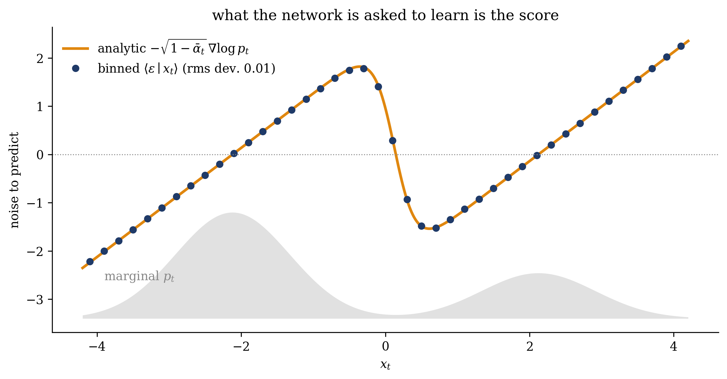
The left half of the box is the loss you trained, one weight away (\(L_\text{simple}\) drops the prefactor — the second engineering decision). The right half is the identity that closes the module’s circle, and it is not an analogy but Week 10 verbatim. The conditional score of the marginal Equation 23.1 is \(\nabla_{x_t} \log q(x_t \mid x_0) = -(x_t - \sqrt{\bar{\alpha}_t}\, x_0)/(1 - \bar{\alpha}_t) = -\varepsilon / \sqrt{1 - \bar{\alpha}_t}\), so the \(\varepsilon\)-regression in Equation 23.5is denoising score matching (Equation 19.4) at noise scale \(\sigma^2 = 1 - \bar{\alpha}_t\), rescaled: by Vincent’s identity its minimizer is \(\varepsilon_\theta^*(x_t, t) = \langle \varepsilon \mid x_t \rangle = -\sqrt{1 - \bar{\alpha}_t}\; \nabla_{x_t} \log q_t(x_t)\), the score of the blurred marginal in different units. The network you trained to guess noise was estimating \(\nabla \log p_t\) all along, and the whole objective is the syllabus sentence made precise: denoising score matching at every noise level, tied together by the variational bound.Figure 23.2 verifies the identity with no training in the loop — the conditional mean of the noise, estimated by binned averages from raw corruption samples, lands on the rescaled analytic score of the running two-mode target.
Figure 23.2: The \(\varepsilon\)-regression target is the rescaled score, verified without training. At noise level \(\bar{\alpha}_t = 0.5\), corruption samples \(x_t = \sqrt{\bar{\alpha}_t}\,x_0 + \sqrt{1-\bar{\alpha}_t}\,\varepsilon\) of the running two-mode target are binned in \(x_t\) and the added noise \(\varepsilon\) is averaged within each bin (navy points, \(4 \times 10^5\) samples, bins with at least 500 hits). The binned conditional mean \(\langle \varepsilon \mid x_t \rangle\) — the minimizer of the DDPM regression Equation 23.5 — lands on the analytic curve \(-\sqrt{1-\bar{\alpha}_t}\,\nabla \log p_t\) (orange) to an rms deviation of \(0.01\). The gray band underneath is the marginal \(p_t\): where the blur has mass the estimate is tight, and the sparse bins near the density minimum scatter visibly — the same coverage effect that Week 10 flagged for learned scores.
Take-home 2
With a fixed-covariance Gaussian ansatz for the reverse kernels, each ledger entry collapses to a squared error between posterior and model means, and in the noise variable to the weighted regression Equation 23.5. Its minimizer is \(\langle \varepsilon \mid x_t \rangle = -\sqrt{1-\bar{\alpha}_t}\,\nabla \log p_t\): the noise-prediction network is a score model in different units, and the DDPM objective is denoising score matching at every rung, held together by the variational bound.
23.5 The engineering ledger
Every remaining feature of the recipe is an engineering decision layered on top of the exact construction. Four entries follow, in the order they appeared.
① Fixed reverse variances.Ho, Jain, and Abbeel (2020) set \(\sigma_t^2\) to \(\beta_t\) or to \(\tilde{\beta}_t\) and report similar results for both. The two are the ends of a bracket — \(\tilde{\beta}_t\) is the posterior variance when \(x_0\) is deterministic, \(\beta_t\) the correct value when \(p_0\) is itself a unit Gaussian — and for the schedules in use they differ by little except at the smallest \(t\). Learning the variances (interpolating inside the bracket) recovers a few hundredths of a nat of likelihood (Nichol and Dhariwal 2021); the mean is where the physics is.
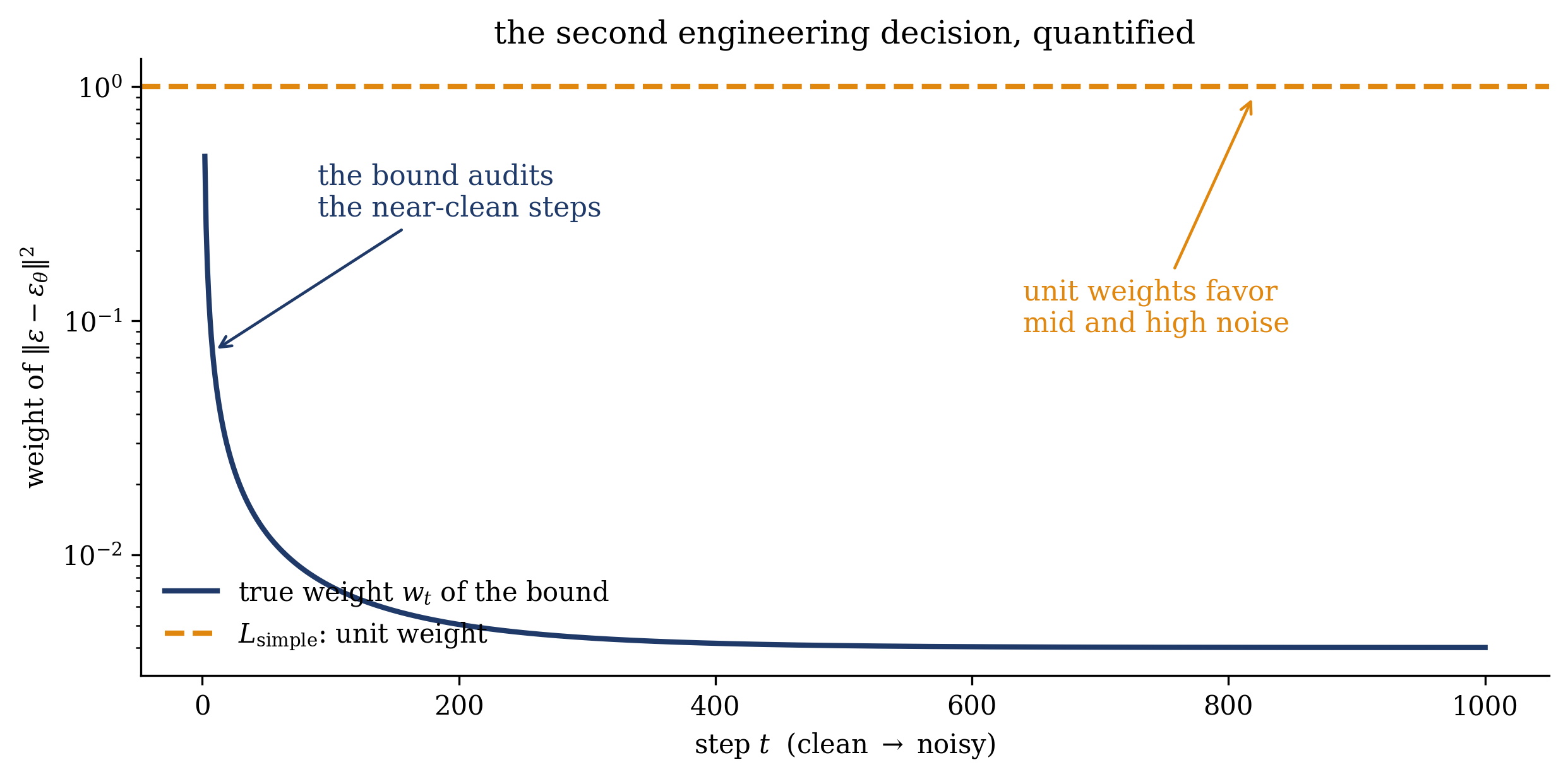
② Unit weights. The full bound Equation 23.5 carries the prefactor \(w_t = \beta_t^2 / \big(2 \sigma_t^2 \alpha_t (1 - \bar{\alpha}_t)\big)\); \(L_\text{simple}\) replaces every \(w_t\) by one. Figure 23.3 computes the true weights for a \(T = 1000\) chain: they span more than two orders of magnitude and concentrate at the near-clean steps, where the bound audits fine detail — exactly the terms that dominate a log-likelihood. Setting them to one down-weights the clean end and spends the network’s capacity at mid and high noise, where the large-scale structure of a sample is decided. The result is a deliberate trade: better perceptual samples, a worse (indeed, no longer guaranteed) likelihood bound. The repair is also known precisely: Song, Durkan, et al. (2021) show that one specific reweighting — the likelihood weighting, \(g^2(t)\) in the continuous-time notation of the next lecture — restores a rigorous upper bound on the negative log-likelihood. The weights are a dial between the two objectives.
③ The schedule, and why \(T \sim 10^3\). The pair (schedule \(\beta_t\), step count \(T\)) is a protocol in Week 11’s sense, and it is priced by Week 11’s laws. The per-step dissipation must be kept small for a reason specific to today’s ansatz: the true one-step reversal \(q(x_{t-1} \mid x_t)\) — without the \(x_0\) anchor — is not Gaussian; it is a mixture as structured as the data themselves, and only in the small-\(\beta_t\) limit does it collapse onto a Gaussian (Sohl-Dickstein et al. 2015). The Gaussian ansatz is therefore not innocent: it is an approximation whose error is controlled by the step size, and the \(1/K\) dissipation law of Section 22.5 is the reason a thousand gentle steps outperform ten abrupt ones at fixed total corruption. The worked example below makes this failure visible on demand.
④ What the network predicts. Regressing \(\varepsilon\), regressing \(x_0\), or regressing the mean \(\mu\) are algebraically interchangeable — each is an affine function of the others given \(x_t\) — but they precondition the network differently: the \(\varepsilon\)-target has unit variance at every \(t\), while an \(x_0\)-target collapses at the clean end and a \(\mu\)-target nearly duplicates the input. Karras et al. (2022) audit these scalings, together with schedules and samplers, as one decoupled design space; the stat-mech construction fixes none of them, and says so.
Figure 23.3: What \(L_\text{simple}\) actually reweights. True per-step weights \(w_t = \beta_t^2/\big(2\sigma_t^2 \alpha_t (1-\bar{\alpha}_t)\big)\) of the bound Equation 23.5 (navy), for a \(T = 1000\) discretization of the Week-10 corruption (\(\sqrt{\bar{\alpha}_t} = e^{-4t/T}\), \(\sigma_t^2 = \tilde{\beta}_t\)), against the unit weight of \(L_\text{simple}\) (orange dashed). The bound concentrates its attention at the near-clean steps — \(w_t \approx 0.50\) at \(t = 2\) against \(0.004\) at \(t = T\), a factor of \(125\), diverging as \(t \to 1\) — because small corruptions carry the fine, likelihood-dominating detail. Replacing \(w_t\) by \(1\) shifts the training effort toward mid and high noise, where perceptual structure is decided: a deliberate engineering trade of likelihood for sample quality.
Trap
The standard misreadings of the DDPM recipe. ① \(L_\text{simple}\) is not a likelihood bound. Dropping the weights \(w_t\) forfeits the inequality of Equation 23.3; reporting \(L_\text{simple}\) (or a naively reweighted variant) as a negative log-likelihood is a category error — the honest bound needs the weights, or the likelihood weighting of Song, Durkan, et al. (2021). ② The Gaussian reverse kernel is an approximation, and the step size is its control parameter. The exact reversal of one corruption step is as multimodal as the data; only small \(\beta_t\) makes it Gaussian. Large steps do not merely coarsen a sound method — they break its central ansatz (Figure 23.4). ③ \(\varepsilon_\theta\) is the score in disguise, units included. Any sampler bolted onto a trained DDPM — Langevin refinement, the reverse SDE, the next lecture’s probability-flow ODE — needs \(s_\theta = -\varepsilon_\theta/\sqrt{1-\bar{\alpha}_t}\); dropping the rescaling is the classic silent bug, wrong by a factor that varies with \(t\).
23.6 Example: the ansatz needs small steps
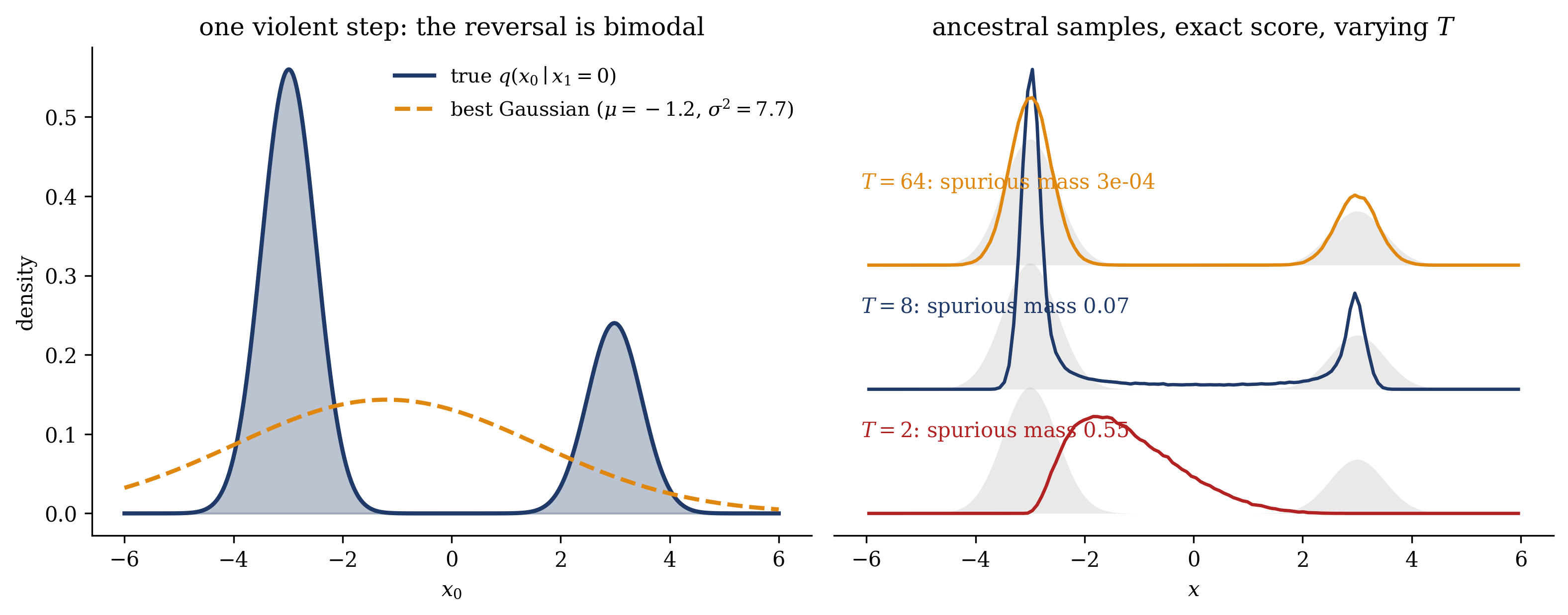
Entry ③ locates the construction’s single structural approximation and merits a demonstration. We use the running two-mode target with its exact scores, so that learning error is zero by construction and whatever fails is the ansatz. The sampler is exactly Ho’s ancestral chain: start at \(x_T \sim \mathcal{N}(0,1)\), step down with \(x_{t-1} = \mu_\theta(x_t, t) + \sigma_t z\) — the mean built from the exact score via Equation 23.5, \(\sigma_t^2 = \tilde{\beta}_t\), no noise on the final step — and vary only the number of steps \(T\) at fixed total corruption (\(\sqrt{\bar{\alpha}_t} = e^{-4t/T}\), as throughout).
Show code
def ancestral(T, n=200_000): tk =4.0* np.arange(T +1) / T ab = np.exp(-2* tk) al = ab[1:] / ab[:-1] be =1- al x = rng.normal(size=n)for t inrange(T, 0, -1): mu = (x + be[t -1] * score_t(x, ab[t])) / np.sqrt(al[t -1])if t >1: bt = (1- ab[t -1]) * be[t -1] / (1- ab[t]) x = mu + np.sqrt(bt) * rng.normal(size=n)else: x = mureturn xfig, (a1, a2) = plt.subplots(1, 2, figsize=(10.6, 4.2))# left: the true one-step reversal at T=2 versus its best Gaussiantk =4.0* np.arange(3) /2ab = np.exp(-2* tk)al0, be0 = ab[1] / ab[0], 1- ab[1] / ab[0]xs = np.linspace(-6, 6, 1200)p0 = (wts * np.exp(-(xs[:, None] - mus)**2/ (2* sigs**2))/ (np.sqrt(2* np.pi) * sigs)).sum(1)post = p0 * np.exp(-(0.0- np.sqrt(al0) * xs)**2/ (2* be0))post /= np.trapz(post, xs)m_post = np.trapz(xs * post, xs)v_post = np.trapz((xs - m_post)**2* post, xs)gauss = np.exp(-(xs - m_post)**2/ (2* v_post)) / np.sqrt(2* np.pi * v_post)a1.fill_between(xs, post, color=NAVY, alpha=0.30)a1.plot(xs, post, color=NAVY, lw=2.0, label=r"true $q(x_0 \mid x_1 = 0)$")a1.plot(xs, gauss, color=ORANGE, lw=2.0, ls="--", label=rf"best Gaussian ($\mu={m_post:.1f}$, $\sigma^2={v_post:.1f}$)")a1.set_xlabel(r"$x_0$"); a1.set_ylabel("density")a1.set_title(r"one violent step: the reversal is bimodal", fontsize=12)a1.legend(frameon=False, fontsize=9.5, loc="upper right")# right: ancestral samples vs step countoffsets = {2: 0.0, 8: 0.55, 64: 1.10}for T, off in offsets.items(): x = ancestral(T) hist, edges = np.histogram(x, bins=140, range=(-6, 6), density=True) cen =0.5* (edges[1:] + edges[:-1]) col = RED if T ==2else (NAVY if T ==8else ORANGE) a2.fill_between(xs, off, off + p0, color=GRAY, alpha=0.18, lw=0) a2.plot(cen, hist + off, color=col, lw=1.6) spur = ((x >-1.5) & (x <1.5)).mean() lab =f"{spur:.2f}"if spur >=0.01elsef"{spur:.0e}" a2.text(-6.1, off +0.34, rf"$T={T}$: spurious mass {lab}", color=col, fontsize=10)a2.set_xlabel(r"$x$")a2.set_yticks([])a2.spines["left"].set_visible(False)a2.set_title("ancestral samples, exact score, varying $T$", fontsize=12)fig.tight_layout()plt.show()
Figure 23.4: The Gaussian ansatz needs small steps — exact scores, so every failure is the ansatz. Left: the true one-step reversal \(q(x_0 \mid x_1)\) for a two-step chain (\(T = 2\), \(\beta_t = 0.98\)), evaluated at \(x_1 = 0\) (navy): it is bimodal with modes at the two data modes and variance \(7.7\), and no Gaussian — the moment-matched one is shown in orange — can represent it. Right: ancestral samples against the true density (gray) for \(T = 2\), \(8\), \(64\) at fixed total corruption. At \(T = 2\) the sampler pours \(55\%\) of its mass into the region \(|x| < 1.5\), which truly holds \(0.001\); at \(T = 8\) the spurious mass is down to \(7\%\); at \(T = 64\) it is \(3 \times 10^{-4}\), with the mode weight at \(0.295\) against the true \(0.300\). The steps must be small enough that the true reversal kernel is Gaussian; a thousand gentle steps is a requirement of the ansatz.
The left panel of Figure 23.4 is the anatomy of the failure. After a two-step corruption each step replaces \(98\%\) of the variance, and the true reversal \(q(x_0 \mid x_1)\) at \(x_1 = 0\) is the data distribution itself, barely tilted: two humps, six units apart. The Gaussian ansatz can place its mean correctly — with the exact score it does, at \(-1.19\), the posterior mean — but a single Gaussian centered between two modes puts its mass where neither mode lives. The right panel shows the consequence and its cure: at \(T = 2\) over half the generated mass lands in the inter-mode region that truly carries \(10^{-3}\) of the probability, and the defect drains away as the steps shrink, three orders of magnitude by \(T = 64\). Nothing was learned or mislearned anywhere in this figure; the error is purely the distance between the true reversal kernel and the Gaussian family, and step size is the only dial that controls it. This is Week 11’s near-equilibrium lesson relocated into a generative model: gentle protocols are the ones whose reversals are simple.
Take-home 3
Four engineering decisions sit on top of the exact construction: fixed reverse variances, unit weights (\(L_\text{simple}\) trades the likelihood bound for sample quality; a specific likelihood weighting restores it (Song, Durkan, et al. 2021)), the schedule with \(T \sim 10^3\) (small steps keep the true reversal Gaussian — the ansatz’s one structural requirement), and the choice of regression target (\(\varepsilon\) for its unit variance at every \(t\)). Everything else is theorem.
A diffusion model trains by minimizing its own dissipation: the DDPM bound is Week 11’s forward/reverse path divergence with the reverse measure made learnable, its per-step ledger is Week 10’s denoising score matching in closed form, and the noise the network predicts is the score in different units.
The warm-up card sends you into the framing sections of Song, Sohl-Dickstein, et al. (2021) — the paper the next lecture is built on — with today’s dictionary in hand: their forward SDE is Equation 20.1, their discrete “DDPM” is today’s chain, and their training loss is Equation 23.5 with a continuous \(t\). The next lecture takes the small-step limit properly — renaming the step index to \(k\), so that \(t\) can become continuous time: the score-SDE framework that unifies today’s chain with Week 10’s continuous picture, the probability-flow ODE — a deterministic sampler with the same marginals and an exact likelihood, no bound required — and a look at flow matching, which reaches the same object without any stochastic construction at all. The tutorial (Ph12 106) then puts the two samplers side by side and connects the likelihood machinery to Week 11’s AIS estimator; the session uses the ledger Equation 23.4 and the reverse SDE Equation 20.2.
23.7 Outlook: one construction, many parametrizations
The lecture decomposed the workhorse of industrial image generation — a method you trained as a recipe — into objects this course built one at a time: a forward corruption chain (Week 10’s Ornstein–Uhlenbeck process, discretized), a variational bound that is a nonequilibrium free-energy estimator (Week 11’s Jensen gap, with the reverse path measure handed to a neural network), per-step terms that are denoising score matching in closed form (Week 10’s regression), and a residue of four engineering decisions whose costs and repairs are each known precisely. The historical lineage is explicit: the founding paper cited Jarzynski before any of deep learning’s own canon.
What the discrete bookkeeping cannot deliver is a likelihood without a bound; that requires the continuous limit. As \(T \to \infty\) the chain converges to the score-SDE of Song, Sohl-Dickstein, et al. (2021), Anderson’s reverse-time SDE returns as the sampler, and a deterministic sibling — the probability-flow ODE — carries the same marginals while permitting exact likelihood evaluation. The partition function that could not be computed in Week 3 has been dodged, bounded, cancelled, removed, measured, and now minimized against, by a model whose training loss is a dissipation.
Ho, Jonathan, Ajay Jain, and Pieter Abbeel. 2020. “Denoising Diffusion Probabilistic Models.” In Advances in Neural Information Processing Systems. Vol. 33. https://arxiv.org/abs/2006.11239.
Karras, Tero, Miika Aittala, Timo Aila, and Samuli Laine. 2022. “Elucidating the Design Space of Diffusion-Based Generative Models.” In NeurIPS. Vol. 35.
Nichol, Alexander Quinn, and Prafulla Dhariwal. 2021. “Improved Denoising Diffusion Probabilistic Models.” In Proceedings of the 38th International Conference on Machine Learning (ICML), PMLR 139, 8162–71.
Sohl-Dickstein, Jascha, Eric Weiss, Niru Maheswaranathan, and Surya Ganguli. 2015. “Deep Unsupervised Learning Using Nonequilibrium Thermodynamics.” In Proceedings of the 32nd International Conference on Machine Learning, 37:2256–65. Proceedings of Machine Learning Research. https://arxiv.org/abs/1503.03585.
Song, Yang, Conor Durkan, Iain Murray, and Stefano Ermon. 2021. “Maximum Likelihood Training of Score-Based Diffusion Models.” In NeurIPS. Vol. 34.
Song, Yang, Jascha Sohl-Dickstein, Diederik P. Kingma, Abhishek Kumar, Stefano Ermon, and Ben Poole. 2021. “Score-Based Generative Modeling Through Stochastic Differential Equations.” In International Conference on Learning Representations. https://arxiv.org/abs/2011.13456.
Welling, Max, Sirui Lu, and Lars Holdijk. 2026. Generative AI and Stochastic Thermodynamics: A Tale of Free Energies. Cambridge: Cambridge University Press. https://doi.org/10.1017/9781009709071.