7 Dense associative memory: the wall was never a law

7.1 The wall was never a law

Recall where Week 2 left associative memory. A network of \(N\) neurons and \(N^2\) Hebbian couplings stores \(\alpha_c N \approx 0.138\,N\) patterns; past that load, retrieval does not degrade but ceases to exist (Section 4.4, Equation 4.6). For decades that number was read as a verdict on the whole idea: associative memory is fundamentally inefficient — a hundred and thirty-eight memories from a million synapses — and the energy-based approach to computation, however beautiful, was capped. The capacity question looked closed, with a disappointing answer.

The verdict was a misreading. The \(0.138\,N\) wall is a property of the particular energy function Hopfield happened to write down, and of nothing else. In 2016, Krotov and Hopfield — Hopfield himself, returning to his own model thirty-four years on — showed that sharpening the energy’s interaction function lifts the capacity to \(N^{n-1}\) for any degree \(n\) (Krotov and Hopfield 2016); a year later, Demircigil et al. (2017) proved that an exponential interaction stores a number of patterns exponential in \(N\), with basins of attraction that remain macroscopic. What set the wall was the shape of the energy function.

The question, then: what set the wall, and how do you move it? Capacity is determined by how sharply each stored pattern’s contribution to the energy is peaked around that pattern. There is a function — the interaction function \(F\) — whose steepness controls this: degree two gives linear capacity, polynomial degree \(n\) gives \(N^{n-1}\), and an exponential gives \(2^{cN}\).

We are still in Module 1, and we have returned to the cold: today’s network is Week 2’s retrieval machine — deterministic, \(T = 0\), couplings written rather than learned, no probabilities and no \(Z\) (the partition function, central in Week 3, plays no role this week; Section 7.6 says precisely why). In the next lecture the scaled-up retrieval rule will turn out to sit at the center of the architecture that now dominates machine learning. One contrast worth noting now: Week 3’s exponential \(2^N\) counted the states in \(Z\) and made training hopeless; this week’s exponential counts the patterns you can store — the same combinatorial explosion, entering with the opposite sign. The ledger below (Section 7.6) makes the comparison quantitative.

Take-home 1

The \(0.138\,N\) capacity is a property of the quadratic Hopfield energy, not of associative memory. Generalize the energy to \(E = -\sum_\mu F(\xi^\mu \cdot s)\) and capacity becomes a dial on the sharpness of \(F\): quadratic gives \(\sim N\), degree \(n\) gives \(\sim N^{n-1}\), exponential gives \(\sim 2^{cN}\). The wall moves — all the way up.

7.2 The model: an energy with a dial

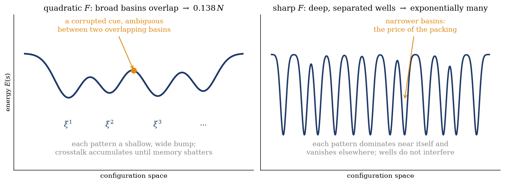
Two pictures organize the lecture, and Figure 7.1 draws them before any formula. In the classical landscape (quadratic energy), each stored pattern contributes a broad, shallow basin. Broad basins overlap; overlapping basins interfere; and Week 2 quantified the interference — a CLT-Gaussian crosstalk of variance \(\alpha\) that drowns the unit signal at \(\alpha_c\) (Equation 4.1). In the dense landscape (sharp interaction), each pattern contributes a deep, narrow well that dominates near itself and dies off elsewhere. Narrow wells do not overlap, so vastly more of them fit before they interfere — and the count will turn out to be exponential. In short: capacity is basin geometry, and the interaction function sets the geometry.

Figure 7.1: The central picture of the lecture: capacity is basin geometry. Left: the quadratic energy of Week 2 — every stored pattern a broad, shallow bump; basins overlap, crosstalk accumulates, and at \(\alpha_c \approx 0.138\) retrieval shatters. A corrupted cue sits ambiguously between neighbors. Right: a sharp interaction function — each pattern a deep, narrow, well-separated well that dominates near itself and vanishes elsewhere; exponentially many fit before they interfere. The price is visible on sight: narrower wells mean smaller basins of attraction, the tradeoff quantified below.

The dense-memory energy. Following Krotov and Hopfield (2016), keep everything from Week 2 — \(N\) binary neurons \(s_i = \pm 1\), \(P\) random stored patterns \(\xi^\mu\), the overlap as the natural variable — and change one thing: how the overlap enters the energy. Define

\[ \boxed{\; E(s) \;=\; -\sum_{\mu=1}^{P} F\big( \xi^\mu \cdot s \big) \;} \tag{7.1}\]

dense-memory energy

where \(\xi^\mu \cdot s = \sum_i \xi_i^\mu s_i\) and \(F\) is a smooth, rapidly growing interaction function (Krotov and Hopfield also say separation function — it separates the matching pattern from the rest, which is exactly the job description). A notation flag, stated once: this \(F\) is not the free energy \(F = -T\log Z\) of Weeks 1 and 3 — an unfortunate but standard collision, confined to this week, and the free energy makes no appearance today to collide with.

The classical model is the quadratic special case, and the script does the one line of algebra: with \(F(x) = x^2/(2N)\),

\[ E \;=\; -\frac{1}{2N} \sum_\mu \big( \xi^\mu \cdot s \big)^2 \;=\; -\frac{1}{2} \sum_{i,j} \underbrace{\Big( \frac{1}{N} \sum_\mu \xi_i^\mu \xi_j^\mu \Big)}_{=\; J_{ij}\ \text{(Hebb, @eq-hebb)}} s_i s_j \;=\; -\frac{1}{2} \sum_{i \neq j} J_{ij}\, s_i s_j \;-\; \frac{P}{2}, \]

Week 2’s Hopfield energy Equation 3.2 up to a constant (the diagonal term, since \(s_i^2 = 1\)). Everything Week 2 proved and computed is the \(F \propto x^2\) row of a bigger table.

The update rule. The dynamics generalizes Week 2’s greedy descent in the only sensible way: flip neuron \(i\) to whichever sign gives the lower energy,

\[ s_i \;\longleftarrow\; \operatorname{sign}\Bigg[ \sum_{\mu} \Big( F\big( \xi^\mu \cdot s \big|_{s_i = +1} \big) - F\big( \xi^\mu \cdot s \big|_{s_i = -1} \big) \Big) \Bigg], \tag{7.2}\]

dense-memory update

asynchronously, one neuron at a time. Two sanity checks, both one line. First, for the quadratic case the bracket collapses (each term is a difference of squares) to \(\propto \sum_\mu \xi_i^\mu \sum_{j \neq i} \xi_j^\mu s_j\) — exactly the local field of Equation 3.1: the classical rule falls out unchanged (Demircigil et al. 2017). Second, the Lyapunov argument of Section 3.4 survives verbatim for any \(F\): the rule flips only when the flip lowers \(E\), configuration space is finite, so the dynamics descends and halts in a local minimum. The landscape picture is a theorem here too.

For smooth \(F\) the bracket linearizes — the two arguments differ by \(\pm 2\xi_i^\mu\) — and the update reads \(s_i \leftarrow \operatorname{sign}(h_i)\) with the effective field

\[ h_i \;=\; \sum_{\mu} F'\big( \xi^\mu \cdot s \big)\, \xi_i^\mu \tag{7.3}\]

effective field: an \(F'\)-weighted vote

— the central object of the analysis. The field is a vote of the stored patterns, exactly as in Week 2 — but now each pattern votes with weight \(F'(\text{its current overlap})\). A steep \(F'\) means the pattern the state currently resembles dominates the vote, and every other pattern barely registers. The interaction function is a filter on the vote, and capacity is decided by how sharply that filter discriminates.

7.3 The engine: signal versus crosstalk, revisited

The derivation repeats Week 2’s signal-versus-crosstalk analysis — the same apparatus, the same CLT, the same Gaussian tails — with \(F'\) now amplifying the signal. In Week 2 the aligned field was \(1 + C_i\) with crosstalk \(C_i \sim \mathcal{N}(0, \alpha)\), and signal barely exceeded crosstalk — the margin vanished at \(\alpha_c\). A steeper \(F'\) widens that margin.

Step 1 — where the two sides live. Put the network at a stored pattern, \(s = \xi^\nu\), and read the effective field Equation 7.3. The matching term has \(\xi^\nu \cdot s = N\): the signal enters through \(F'(N)\). Every other overlap \(\xi^\mu \cdot s\) (\(\mu \neq \nu\)) is a sum of \(N\) independent fair signs — Week 2’s CLT once more — so it is Gaussian of mean zero and width \(\sqrt{N}\): the crosstalk enters through \(F'\big(\mathcal{O}(\sqrt{N})\big)\). The two sides of the contest sit at different arguments of the same function,

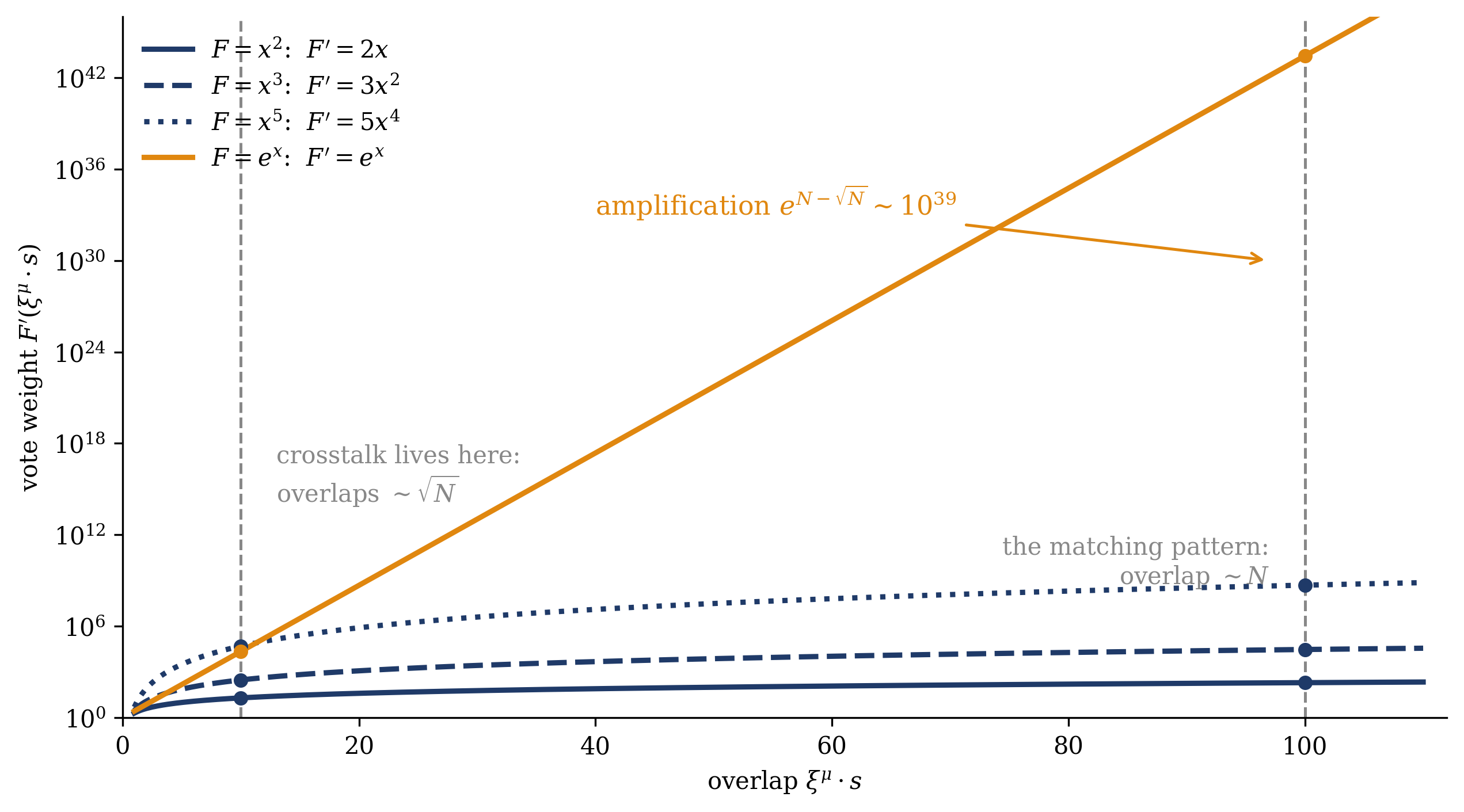
\[ h_i \;=\; \underbrace{F'(N)\, \xi_i^\nu}_{\text{signal}} \;+\; \underbrace{\sum_{\mu \neq \nu} F'\big( \xi^\mu \cdot s \big)\, \xi_i^\mu}_{\text{crosstalk, arguments } \sim \sqrt{N}}, \]

and the signal-to-crosstalk ratio is governed by the amplification factor \(F'(N) / F'(\sqrt{N})\). Figure 7.2 draws it for several choices: for the quadratic, \(F' = 2x\) is a straight line and the factor is a modest \(\sqrt{N}\) — the marginal separation of Week 2. For \(F = x^n\) the factor is \(N^{(n-1)/2}\); for \(F = e^x\) it is \(e^{N - \sqrt{N}}\), already \(\sim 10^{39}\) at \(N = 100\).

Show code

N = 100
x = np.linspace(1, 110, 500)
fig, ax = plt.subplots(figsize=(8.6, 4.8))
curves = [(2 * x, r"$F=x^2$:  $F'=2x$", NAVY, "-"),
          (3 * x**2, r"$F=x^3$:  $F'=3x^2$", NAVY, "--"),
          (5 * x**4, r"$F=x^5$:  $F'=5x^4$", NAVY, ":"),
          (np.exp(x), r"$F=e^x$:  $F'=e^x$", ORANGE, "-")]
for y, lab, c, ls in curves:
    ax.semilogy(x, y, color=c, ls=ls, lw=2.2, label=lab)
for xv, lab, xt, yt, halign in [
        (np.sqrt(N), "crosstalk lives here:\noverlaps $\\sim\\sqrt{N}$", 13, 1e18, "left"),
        (N, "the matching pattern:\noverlap $\\sim N$", 97, 1e12, "right")]:
    ax.axvline(xv, color=GRAY, ls="--", lw=1.2)
    ax.text(xt, yt, lab, color=GRAY, fontsize=10, va="top", ha=halign)
for xv in [np.sqrt(N), N]:
    for y, _, c, _ in curves:
        ax.plot([xv], [np.interp(xv, x, y)], "o", color=c, ms=5)
ax.annotate(r"amplification $e^{N-\sqrt{N}} \sim 10^{39}$",
            xy=(97, 1e30), xytext=(40, 1e33), color=ORANGE, fontsize=11,
            arrowprops=dict(arrowstyle="->", color=ORANGE, lw=1.2))
ax.set_xlabel(r"overlap $\xi^\mu \cdot s$")
ax.set_ylabel(r"vote weight $F'(\xi^\mu\cdot s)$")
ax.set_xlim(0, 112); ax.set_ylim(1, 1e46)
ax.legend(frameon=False, fontsize=10, loc="upper left")
fig.tight_layout(); plt.show()

Figure 7.2: The interaction function as a filter, drawn for a network of \(N = 100\) neurons. The derivative \(F'(x)\) weights each stored pattern’s vote in the effective field Equation 7.3; the crosstalk patterns sit at overlaps \(\sim \sqrt{N} = 10\) (left dashed line) while the matching pattern sits at overlap \(N = 100\) (right dashed line). The signal-to-crosstalk amplification is the vertical gap between the two operating points: a factor \(\sqrt{N} = 10\) for the quadratic (the close contest of Week 2), \(N = 100\) for the cubic, \(10^4\) for degree five — and thirty-nine orders of magnitude for the exponential. The capacity laws of Equation 7.4 are this plot, read off.

Step 2 — the bookkeeping. The scaling argument becomes a capacity number exactly the way it did in Week 2: compute the mean and variance of the stability margin, and ask when the Gaussian tail leaks past zero. Following Krotov and Hopfield (2016), take \(F(x) = x^n\) and ask whether bit \(i\) of the stored pattern \(\xi^\nu\) holds — that is, compare the energy of \(s = \xi^\nu\) against the energy with bit \(i\) flipped. The matching term supplies the energy gap (the signal):

\[ \langle \Delta E \rangle \;=\; N^n - (N - 2)^n \;\approx\; 2n\, N^{n-1}, \]

while each of the \(P - 1\) crosstalk terms shifts by \(\approx \mp 2n\, (\xi^\mu \cdot s)^{n-1}\) with \(\xi^\mu \cdot s \sim \mathcal{N}(0, N)\). Their fluctuation is set by a Gaussian moment — \(\big\langle z^{2(n-1)} \big\rangle = (2n - 3)!!\, N^{n-1}\) for \(z \sim \mathcal{N}(0, N)\), which is where the double factorial that decorates every formula in this field comes from — so the crosstalk variance is

\[ \Sigma^2 \;=\; 4 n^2\, (2n - 3)!!\, (P - 1)\, N^{n-1}. \]

The bit destabilizes when the crosstalk fluctuation beats the gap, which happens with the Gaussian tail probability

\[ P_\text{err} \;=\; \tfrac{1}{2} \operatorname{erfc}\!\big( x / \sqrt{2} \big), \qquad x \;=\; \frac{\langle \Delta E \rangle}{\Sigma} \;=\; \sqrt{ \frac{N^{n-1}}{(2n - 3)!!\; P} }. \]

As a consistency check: \(n = 2\) gives \((2n-3)!! = 1\) and \(x = \sqrt{N/P} = 1/\sqrt{\alpha}\) — exactly the first-sweep error rate Equation 4.2, constant and all. The machinery is identical; only the exponent has changed.

Step 3 — read off the capacity laws. Fix a tolerated per-bit error (retrieval with a small dressing of wrong bits, Week 2’s tolerant question): then \(x = \mathcal{O}(1)\), i.e. \(P \sim N^{n-1}\). Demand instead that every bit of every pattern hold — the strict question — and the union bound over \(NP\) bits costs the usual extreme-value logarithm (Section 4.3, the identical move): \(x^2 \approx 2\ln(NP)\), i.e. \(P \sim N^{n-1}/\big(2 (2n-3)!! \ln N\big)\) (Krotov and Hopfield 2016). And for the exponential interaction \(F(x) = e^x\), the amplification \(F'(N)/F'(\sqrt{N}) = e^{N - \sqrt{N}}\) suppresses the crosstalk to the point that the capacity is exponential — the result Demircigil et al. (2017) made a theorem: storing \(P = e^{\alpha N}\) patterns, every one is a fixed point of the dynamics with probability \(\to 1\) for any \(\alpha < \ln 2 / 2\), i.e. up to

\[ \boxed{\; P_\text{max} \sim \begin{cases} \alpha_c\, N & F = x^2 \quad \text{(Week 2's wall — recovered, not repealed)}\\[4pt] \alpha_n\, N^{\,n-1} & F = x^n \quad \text{[@krotov2016]}\\[4pt] e^{\alpha N},\ \alpha < \tfrac{\ln 2}{2}\ \Rightarrow\ \sim 2^{N/2} & F = e^x \quad \text{[@demircigil2017]} \end{cases} \;} \tag{7.4}\]

the capacity laws

One caveat, inherited from Week 2. These estimates are first-sweep, no-feedback statements — precisely the kind that Section 4.4 showed cannot locate the classical transition, where the errors’ feedback moved the answer from \(2/\pi\) to \(0.138\) and changed its character. For \(n = 2\), then, read the first row as the scaling with the correct constant imported from the self-consistent theory. For \(n > 2\) the situation genuinely improves: the crosstalk suppression is now polynomial or exponential rather than marginal, the union-bound argument can be made rigorous — Demircigil et al. (2017) prove both the polynomial law (with \(c_n > 2(2n-3)!!\)) and the exponential one as theorems — and the first-sweep logic is, for once, the whole story.

⇒ The linear derivative \(F' = 2x\) is what made the classical capacity linear. Any \(F\) whose derivative grows faster lets the matching pattern dominate the crosstalk: polynomial sharpness gives polynomial capacity, exponential sharpness gives exponential capacity.

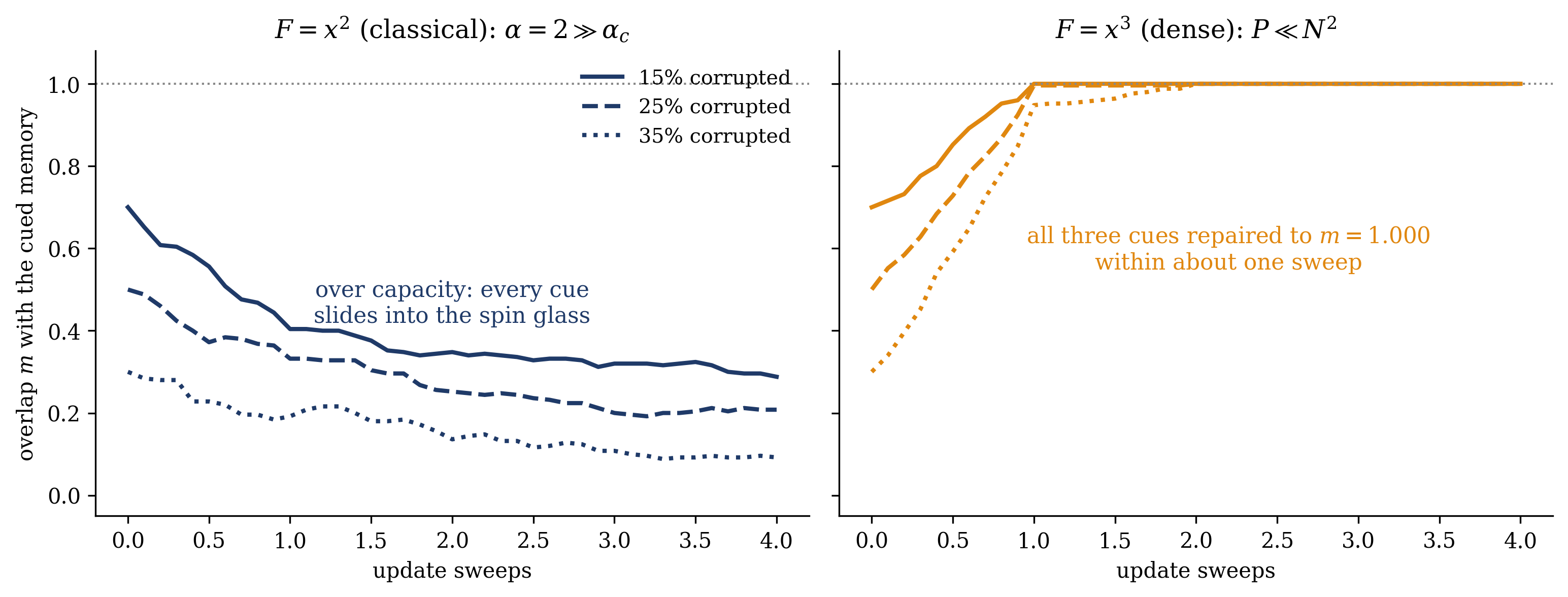
Figure 7.3 confirms the scaling numerically: a network of \(N = 500\) neurons loaded with \(P = 1000\) patterns — load \(\alpha = 2\), fourteen times past the classical wall — cued with corrupted memories under the classical update and under the cubic dense update Equation 7.2. The quadratic network, far past its capacity, drifts into the spin-glass phase from any starting point. The cubic network repairs a \(35\%\)-corrupted cue to \(m = 1.000\) in about one sweep.

Show code

N, P = 500, 1000
rng = np.random.default_rng(4)
X = rng.choice([-1.0, 1.0], size=(P, N))

def retrieve(n_power, f, sweeps=4, record_every=50):
    s = X[0].copy()
    flip = rng.choice(N, size=int(f * N), replace=False)
    s[flip] *= -1
    o = X @ s                                    # running overlaps xi^mu . s
    t, ms = [0.0], [o[0] / N]
    F = lambda x: x**n_power
    for sw in range(sweeps):
        for step, i in enumerate(rng.permutation(N)):
            op = o + X[:, i] * (1 - s[i])        # overlaps with s_i = +1
            om = o - X[:, i] * (1 + s[i])        # overlaps with s_i = -1
            si = 1.0 if (F(op) - F(om)).sum() > 0 else -1.0
            if si != s[i]:
                o += X[:, i] * (si - s[i])
                s[i] = si
            if (step + 1) % record_every == 0:
                t.append(sw + (step + 1) / N); ms.append(o[0] / N)
    return t, ms

fig, axes = plt.subplots(1, 2, figsize=(10.4, 4.0), sharey=True)
for ax, n_power, title in zip(axes, [2, 3],
                              [r"$F = x^2$ (classical): $\alpha = 2 \gg \alpha_c$",
                               r"$F = x^3$ (dense): $P \ll N^2$"]):
    for f, ls in zip([0.15, 0.25, 0.35], ["-", "--", ":"]):
        t, ms = retrieve(n_power, f)
        col = NAVY if n_power == 2 else ORANGE
        ax.plot(t, ms, ls=ls, color=col, lw=2.0, label=rf"{int(f*100)}% corrupted")
    ax.axhline(1.0, color=GRAY, ls=":", lw=1)
    ax.set_title(title, fontsize=12)
    ax.set_xlabel("update sweeps"); ax.set_ylim(-0.05, 1.08)
axes[0].set_ylabel(r"overlap $m$ with the cued memory")
axes[0].text(2.0, 0.42, "over capacity: every cue\nslides into the spin glass",
             color=NAVY, fontsize=10.5, ha="center")
axes[1].text(2.2, 0.55, r"all three cues repaired to $m = 1.000$"
             "\nwithin about one sweep", color=ORANGE, fontsize=10.5, ha="center")
axes[0].legend(frameon=False, fontsize=9.5, loc="upper right")
fig.tight_layout(); plt.show()

Figure 7.3: The capacity laws, run rather than stated: \(N = 500\) neurons, \(P = 1000\) stored patterns — load \(\alpha = 2\), fourteen times the classical wall \(\alpha_c \approx 0.138\) — cued with a stored pattern corrupted in \(15\%\), \(25\%\), and \(35\%\) of its bits, under asynchronous energy-descent updates Equation 7.2. Left: the quadratic interaction (classical Hopfield, \(\sim N\) capacity): far over capacity, every cue drifts away from the memory into the spin-glass phase. Right: the cubic interaction (\(\sim N^2\) capacity, comfortably sufficient for \(P = 10^3 \ll N^2/(2 \cdot 3!! \ln N) \approx 7 \times 10^3\)): every cue is repaired to \(m = 1.000\) within about a sweep. Same neurons, same patterns, same dynamics — only the interaction function differs.

7.4 The price: capacity against robustness

Exponential capacity raises the obvious question: if a sharper \(F\) simply stores more, why would anyone ever use anything but \(F = e^x\)? The answer is visible in Figure 7.1: the deep, narrow well that lets a pattern ignore its neighbors is also a well that a corrupted cue can miss. Sharpening \(F\) shrinks the basins of attraction, and a memory with no basin is a lookup table that demands the exact key.

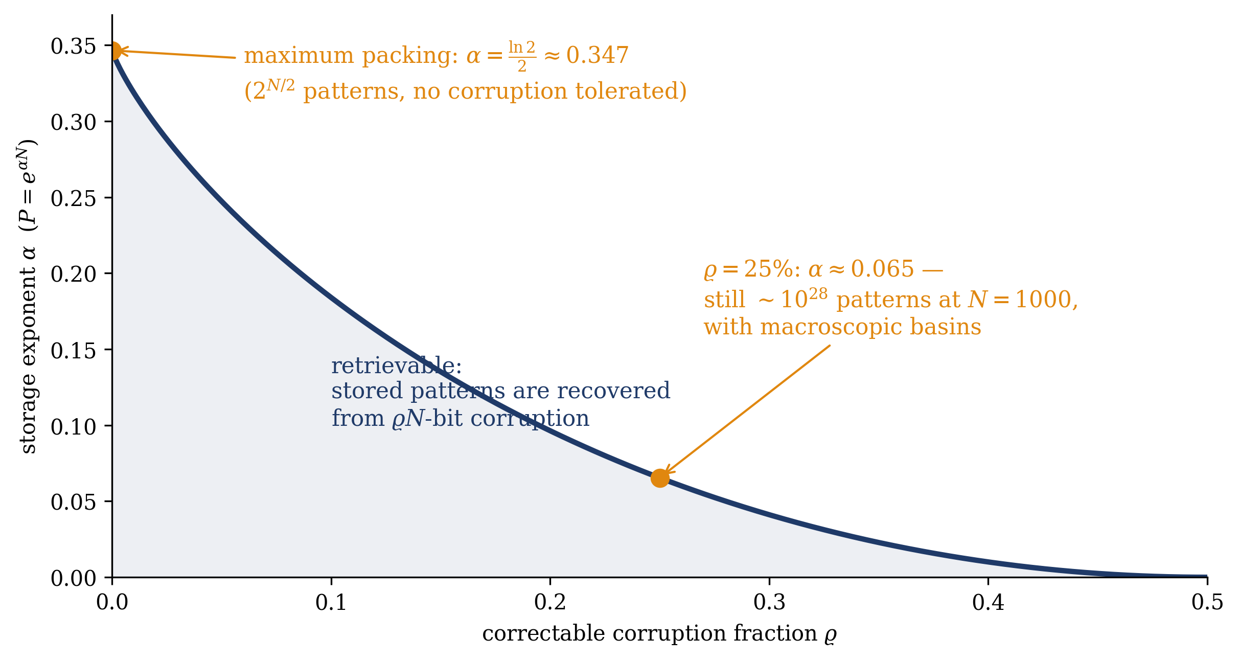
For the exponential model the tradeoff admits an exact formula. The theorem of Demircigil et al. (2017) is quantitative on exactly this point: storing \(P = e^{\alpha N}\) patterns, a cue corrupted in a fraction \(\varrho\) of its bits is repaired (in one step of the dynamics, with probability \(\to 1\)) provided

\[ \alpha \;<\; \frac{I(1 - 2\varrho)}{2}, \qquad I(x) = \tfrac{1}{2}\big[ (1+x)\log(1+x) + (1-x)\log(1-x) \big] \tag{7.5}\]

the capacity–robustness trade curve

— a strictly decreasing function of \(\varrho\). Figure 7.4 plots the curve, and it makes the tradeoff quantitative. At \(\varrho \to 0\) (stability only, no error-correction demanded) the storage exponent reaches its maximum \(I(1)/2 = \ln 2/2 \approx 0.347\): the full \(2^{N/2}\). Demand that the memory still repair \(25\%\) corruption and the exponent drops to \(I(1/2)/2 \approx 0.065\) — at \(N = 1000\) still a comfortable \(\sim 10^{28}\) patterns, which is the content of the paper’s title: huge capacity with macroscopic basins. But push the storage toward its ceiling and the correctable fraction is squeezed to zero: at maximum packing, the wells are pinpricks. Capacity and robustness are two ends of one rope.

Show code

rho = np.linspace(0, 0.4999, 400)
def I(x):
    x = np.atleast_1d(np.asarray(x, dtype=float))
    lo = np.zeros_like(x)                       # (1-x) log(1-x) -> 0 as x -> 1
    m = x < 1
    lo[m] = (1 - x[m]) * np.log1p(-x[m])
    return 0.5 * ((1 + x) * np.log1p(x) + lo)
alpha = I(1 - 2 * rho) / 2
fig, ax = plt.subplots(figsize=(8.2, 4.4))
ax.plot(rho, alpha, color=NAVY, lw=2.5)
ax.fill_between(rho, 0, alpha, color=NAVY, alpha=0.08)
ax.text(0.10, 0.10, "retrievable:\nstored patterns are recovered\nfrom $\\varrho N$-bit corruption",
        color=NAVY, fontsize=10.5)
ax.plot([0], [np.log(2) / 2], "o", color=ORANGE, ms=8)
ax.annotate(r"maximum packing: $\alpha = \frac{\ln 2}{2} \approx 0.347$"
            "\n($2^{N/2}$ patterns, no corruption tolerated)",
            xy=(0, np.log(2) / 2), xytext=(0.06, 0.315), color=ORANGE, fontsize=10.5,
            arrowprops=dict(arrowstyle="->", color=ORANGE, lw=1))
ax.plot([0.25], [I(0.5) / 2], "o", color=ORANGE, ms=8)
ax.annotate(r"$\varrho = 25\%$: $\alpha \approx 0.065$ —"
            "\nstill $\\sim 10^{28}$ patterns at $N = 1000$,"
            "\nwith macroscopic basins",
            xy=(0.25, I(0.5) / 2), xytext=(0.27, 0.16), color=ORANGE, fontsize=10.5,
            arrowprops=dict(arrowstyle="->", color=ORANGE, lw=1))
ax.set_xlabel(r"correctable corruption fraction $\varrho$")
ax.set_ylabel(r"storage exponent $\alpha$  ($P = e^{\alpha N}$)")
ax.set_xlim(0, 0.5); ax.set_ylim(0, 0.37)
fig.tight_layout(); plt.show()

Figure 7.4: The capacity–robustness tradeoff for the exponential interaction, exactly, from Equation 7.5: the largest storage exponent \(\alpha\) (capacity \(P = e^{\alpha N}\)) compatible with repairing a cue corrupted in a fraction \(\varrho\) of its bits. At \(\varrho = 0\) the exponent reaches \(\ln 2/2 \approx 0.347\) — the full \(2^{N/2}\), with no error-correction to spare. At \(\varrho = 0.25\) the exponent is \(\approx 0.065\): still \(\sim 10^{28}\) patterns at \(N = 1000\), with genuinely macroscopic basins. As \(\varrho \to 1/2\) (a cue barely better than chance) the storable exponent vanishes. More memories or wider basins — the dial buys one with the other.

The same rope runs along the polynomial family, in a form Krotov and Hopfield turned from bug into insight. At small \(n\), each stored pattern’s well is broad, and the network’s fixed points blend nearby training examples — retrieval lands on something like a class average. At large \(n\), wells are narrow and private — retrieval lands on the individual example. Krotov and Hopfield call the two ends feature-matching and prototype regimes, and demonstrate on real data (MNIST digits) that the network’s character — what kind of representation it learns, how it generalizes, how it errs — changes qualitatively along the dial (Krotov and Hopfield 2016). The interaction function does more than set capacity: it selects what kind of memory you have: a few robust, heavily-averaged attractors, or a vast archive of brittle individual ones. Spurious mixture states, Week 2’s uninvited guests, populate the low-\(n\) end and thin out with sharpness — and the averaging they perform, useless for exact recall, is precisely what starts to look like generalization at the feature end. The next lecture develops this connection.

Trap

Exponential capacity is not a free lunch. Sharpening \(F\) multiplies the wells and narrows every one of them: the correctable corruption shrinks as the storage exponent grows, with Equation 7.5 the exact exchange rate. A network holding \(2^{N/2}\) patterns at maximum packing forgives essentially no corruption — capacity and robustness must always be quoted together.

Take-home 2

The dial has a price: sharper \(F\) means deeper, narrower basins — more memories, weaker error-correction, with the exact trade curve \(\alpha < I(1 - 2\varrho)/2\) for the exponential case. Along the polynomial family the same rope shows as Krotov–Hopfield’s feature-vs-prototype regimes: broad wells average examples (generalize), narrow wells archive them (memorize). Choose \(F\) for the task.

7.5 Toward the next lecture: continuous states, one-step retrieval

Consider once more the exponential filter: \(F' = e^x\) weights each stored pattern by the exponential of its overlap, so the effective field is dominated — by the factor \(\sim 10^{39}\) of Figure 7.2 at \(N = 100\) — by the single best-matching pattern. The exponential interaction is a smooth implementation of “return the nearest stored memory,” and the sum over patterns in Equation 7.3 is, in disguise, a soft maximum over overlaps. Varying the steepness with an inverse-temperature-like parameter interpolates between exact one-winner retrieval and the averaging of the prototype regime.

The next lecture takes this energy and makes two moves. The states become continuous vectors rather than \(\pm 1\) spins — the energy built on the log-sum-exp of the overlaps, the smooth soft-maximum function — and retrieval, which today takes a sweep of single-spin flips, collapses to essentially one step: a single update carries a query to (a soft average of) the matching stored pattern, with a sharpness parameter \(\beta\) tuning exact retrieval against averaging (Ramsauer et al. 2021). That update rule is the subject of the next lecture — and it is one you have seen before, under another name.

All of this week’s sums run over the \(P\) stored patterns — and even \(2^{N/2}\) of them is a sum you index, not the \(2^N\) sum over configurations that constitutes \(Z\). Today’s normalizations live in Week 1’s tractable regime (a softmax over a finite menu, like the classifier of Section 1.6); nothing here needs, or computes, a partition function. \(Z\) is absent this week because retrieval never requires it; it returns when an energy must represent a normalized distribution — Week 3’s problem, and Module 2’s.

7.6 Example: the capacity ledger, and a familiar number

One network — \(N = 1000\) neurons, the size Week 2’s ledger used — and every capacity law of Equation 7.4 evaluated on it. The printed numbers are the pure scaling laws; the constants of Krotov and Hopfield (2016) (\(\alpha_n\), the double factorial, the strict-stability logarithm) trim one to two orders of magnitude off the polynomial rows, which at this table’s scale is a rounding error.

interaction \(F\)	capacity law	\(P_\text{max}\) at \(N = 1000\)	basins
\(x^2\) (classical)	\(\alpha_c N\)	\(\approx 138\)	wide; robust recall
\(x^3\)	\(\sim N^2\)	\(\sim 10^6\)	narrower
\(x^5\)	\(\sim N^4\)	\(\sim 10^{12}\)	narrower still
\(e^x\)	\(\sim 2^{N/2}\)	\(\sim 3 \times 10^{150}\)	macroscopic if \(\alpha\) backs off the ceiling (Equation 7.5)

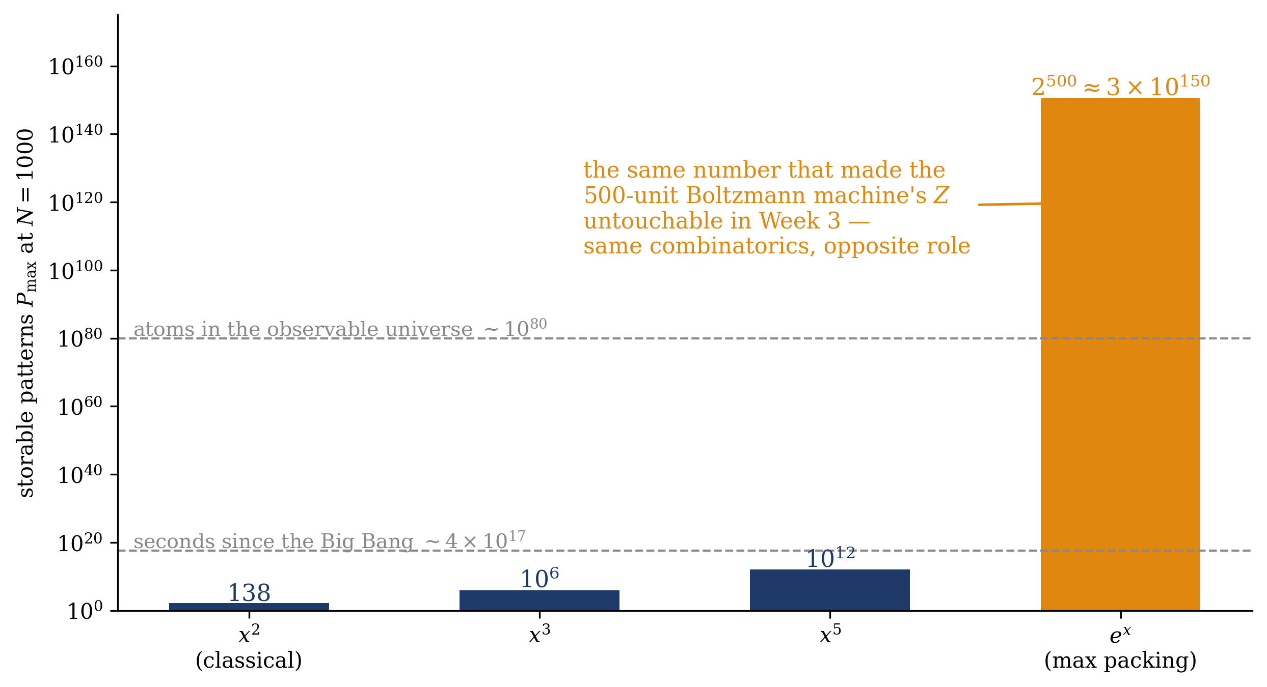
The last row’s number appeared before. In Week 3’s ledger (Section 5.7), a Boltzmann machine of \(500\) units had a partition function of \(2^{500} \approx 3 \times 10^{150}\) terms — more than the atoms of the observable universe, the number that made training hopeless. Today, a memory of \(1000\) neurons stores \(2^{500}\) patterns — numerically the same. The coincidence is structural: the exponential explosion of configuration space enters the denominator when you must normalize (Week 3’s problem) and the capacity when you get to store into it. Same combinatorics, opposite role. Figure 7.5 draws the four bars, with Week 3’s comparators kept deliberately in frame.

Show code

labels = [r"$x^2$" "\n(classical)", r"$x^3$", r"$x^5$", r"$e^x$" "\n(max packing)"]
vals = [138, 1e6, 1e12, 2.0**500]
fig, ax = plt.subplots(figsize=(8.4, 4.6))
bars = ax.bar(labels, vals, color=[NAVY, NAVY, NAVY, ORANGE], width=0.55)
ax.set_yscale("log")
for lv, lab in [(4.4e17, r"seconds since the Big Bang $\sim 4\times10^{17}$"),
                (1e80, r"atoms in the observable universe $\sim 10^{80}$")]:
    ax.axhline(lv, color=GRAY, ls="--", lw=1)
    ax.text(-0.4, lv * 8, lab, color=GRAY, fontsize=9.5)
for i, v in enumerate(vals):
    txt = "138" if i == 0 else (r"$10^{6}$" if i == 1 else (r"$10^{12}$" if i == 2
          else r"$2^{500} \approx 3\times10^{150}$"))
    ax.text(i, v * 8, txt, ha="center", color=NAVY if i < 3 else ORANGE, fontsize=11)
ax.annotate("the same number that made the\n500-unit Boltzmann machine's $Z$\nuntouchable in Week 3 —\nsame combinatorics, opposite role",
            xy=(3, 1e120), xytext=(1.15, 1e105), color=ORANGE, fontsize=10.5,
            arrowprops=dict(arrowstyle="->", color=ORANGE, lw=1.2))
ax.set_ylabel(r"storable patterns $P_\mathrm{max}$ at $N = 1000$")
ax.set_ylim(1, 1e175)
fig.tight_layout(); plt.show()

Figure 7.5: The capacity ledger at \(N = 1000\), on the log scale it demands. Four interaction functions, four capacity laws: \(138\) patterns (quadratic — Week 2’s wall), \(\sim 10^6\) (cubic), \(\sim 10^{12}\) (degree five), \(\sim 3 \times 10^{150}\) (exponential, at maximum packing \(2^{N/2}\)). The gray comparators are kept from Week 3’s ledger on purpose: the exponential memory stores more patterns than there are atoms in the observable universe — and its capacity, \(2^{500}\), is numerically *identical* to the count of terms that made the \(500\)-unit Boltzmann machine’s partition function untouchable. Same combinatorics, opposite role.

The fourth column qualifies the third. Beside every capacity, its basin: the quadratic network at low load repaired a \(49\%\)-corrupted cue (Section 3.6); the exponential network at maximum packing repairs essentially nothing, and buying back a \(25\%\) basin costs the exponent a factor of five. The two columns move in opposite directions and should always be read together.

Practical pointers for the week: the warm-up card (due the evening before the next lecture) works from this lecture and the two capacity papers — you will run the \(F'\) filter argument yourself on a case the lecture did not do, and meet the tradeoff quantitatively. In the next lecture we make the states continuous and the retrieval collapses to a single step — and the rule that does it is one you will recognize the instant you see it written as a matrix product. The tutorial is derivation-led: the hard problem is cracked at the board. The session is device-free.

The \(0.138\,N\) wall was a fact about a quadratic, not about memory — sharpen the energy and it moves without limit.

Take-home 3

At \(N = 1000\): the quadratic memory holds \(138\) patterns, the cubic a million, the exponential \(2^{500} \approx 3 \times 10^{150}\) — numerically the same count of states that made Week 3’s partition function hopeless. The exponential explosion enters the denominator when you must normalize (Week 3) and the capacity when you store into it (Week 4) — same combinatorics, opposite role.

7.7 Outlook: Module 1 closes

Module 1 is now complete. Week 2 designed an energy: memory as attractors, one shot of Hebb, capacity capped at \(0.138\,N\), with \(Z\) absent because nothing was normalized. Week 3 learned an energy: the same network heated up became a probability model, and the instant its couplings were fit by likelihood, \(\nabla_\theta \log Z\) rose as the training obstruction — a sum over \(2^N\) states. Week 4 scaled the energy: back in the cold, a sharper interaction function moved the capacity wall from \(138\) to beyond the atoms of the universe, and \(Z\) dropped out again because retrieval only ever normalizes over the stored patterns. In the next lecture the scaled-up retrieval rule turns out to be the transformer’s own retrieval mechanism — and the 2024 Nobel’s two halves meet in a single equation.

Module 2 begins when we ask an energy model to represent a distribution rather than retrieve a pattern — there the normalizer is \(2^N\) again, non-negotiably, and mean-field and variational methods are the first principled machinery for taming it by bounding it rather than dodging it as Week 3 did. Week 10 remains the standing promise: \(\nabla_x \log Z = 0\) dissolves the negative phase outright, the resolution that every intervening module’s approximation postpones. The two derivatives — with respect to parameters and with respect to inputs — remain distinct.