13 Hubbard–Stratonovich: interactions become latent variables

13.1 Remove the interaction, don’t approximate it

Module 2 has so far worked around the intractable interacting distribution. Week 5 bounded it, restricting the variational family to factorized distributions and accepting the gap Equation 9.1 as the price; Week 6 corrected the bound’s blindness with the reaction term of Chapter 11 and then reorganized the whole computation into messages on a graph (Chapter 12). All three methods live with the interaction and manage its consequences. Today we do something categorically different: we remove the interaction — exactly. A one-line Gaussian identity trades the coupling between spins for a coupling of each spin to a single shared auxiliary field, so that the interacting problem becomes an independent-spin problem at the price of one ordinary integral. No approximation is made anywhere.

The identity is the Hubbard–Stratonovich transformation, and its history runs through two short papers a world apart: Stratonovich (1957), in the Soviet literature on quantum distribution functions, and Hubbard (1959), who used it to rewrite partition functions of interacting systems as functional integrals over auxiliary fields — the move that became the daily workhorse of quantum field theory, where “integrating in a field” is how interacting particles become field theories in the first place. Machine learning, meanwhile, built the same structure from the opposite shore without knowing it: mixture models, factor analysis, and the EM algorithm of Dempster, Laird, and Rubin (1977) all posit a hidden variable \(z\) whose value renders the observations independent, and fit it to data. Today’s lecture proves that these are one construction. The auxiliary field that decouples an interacting system is a latent variable, and a latent-variable generative model is an interacting system with the interaction integrated out.

The driving question follows: what is the auxiliary field, really? It enters as a bare integration variable — introduced by hand, with no physical meaning of its own. Yet by the end of Section 13.3 its saddle-point value will be the magnetization, Week 5’s order parameter, satisfying Week 5’s equation; and by the end of Section 13.4 the field itself will be the latent variable of a generative model, with a prior, a conditional, and a graphical model attached. One object serves two communities, and the transformation is the dictionary between them. Where Week 5 derived mean field as a variational bound, today derives the same equation as the leading order of something exact — which is why mean field is simultaneously an approximation and the beginning of a systematic truth, and why its corrections were computable at all.

Take-home 1

The Hubbard–Stratonovich transformation removes an interaction exactly: interacting spins become independent spins in a single shared auxiliary field, at the cost of one integral. That auxiliary field is both the physicist’s order parameter (its saddle value is the magnetization) and the machine-learner’s latent variable (the hidden common cause of the observations) — the same object, seen from two shores.

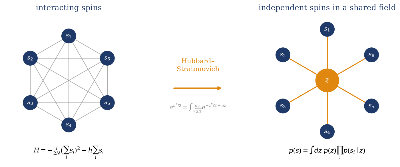
Figure 13.1 shows the central picture: a fully connected graph of interacting spins collapses to a star, every spin attached only to a central auxiliary node \(z\), with no spin–spin edge surviving. The left half is Week 5’s problem; the right half is, literally, the graphical model of a latent-variable generative model. The mathematics below is the proof that the arrow between them is an equality.

Figure 13.1: The lecture in one picture. Left: the Curie–Weiss ferromagnet — every spin coupled to every other through \((\sum_i s_i)^2\), the all-to-all interaction that makes \(Z\) a sum over \(2^N\) coupled configurations. Right: the same model after the Hubbard–Stratonovich transformation — each spin couples *linearly and independently* to one shared auxiliary field \(z\), and no spin–spin edge remains. The star graph is exactly the graphical model of a latent-variable generative model: observations conditionally independent given a hidden common cause.

13.2 The engine: decoupling by a Gaussian

Setup. We work on the model where the transformation is cleanest: the Curie–Weiss ferromagnet of Section 10.2, fully connected with \(J_{ij} = J/N\) and \(J > 0\), in a field \(h\). Its Hamiltonian is a perfect square,

\[ H \;=\; -\frac{J}{2N} \Big( \sum_i s_i \Big)^{2} \;-\; h \sum_i s_i, \qquad\text{so}\qquad Z \;=\; \sum_{\{s\}} \exp\!\left[ \frac{\beta J}{2N} \Big( \sum_i s_i \Big)^{2} + \beta h \sum_i s_i \right]. \]

The obstacle is the square: expanded, \((\sum_i s_i)^2 = \sum_{ij} s_i s_j\) couples every spin to every other, and the sum over \(\{s\}\) does not factorize. Everything Week 5 and Week 6 did was a strategy for living with that square. The question is: can a square be traded for something linear?

The identity. It can, and the tool is one we have carried since Week 1. Complete the square in the exponent of a Gaussian integral: \(-\tfrac{z^2}{2} + a z = -\tfrac{(z - a)^2}{2} + \tfrac{a^2}{2}\), so by Equation 2.1 (shift \(z \to z + a\), which sweeps out the same real line),

\[ \boxed{\; e^{a^{2}/2} \;=\; \frac{1}{\sqrt{2\pi}} \int_{-\infty}^{\infty} \mathrm{d}z\; e^{-z^{2}/2 \,+\, a z} \;} \tag{13.1}\]

Hubbard–Stratonovich identity

Read it as a trade: on the left, the square of a quantity \(a\); on the right, \(a\) appears only linearly, coupled to a new integration variable \(z\) that is averaged over a Gaussian. If \(a\) is a sum over spins, its square couples them all — but a linear term does not couple anything. The identity converts an interaction into an average over fields, exactly. (This is Week 1’s Gaussian integral run in reverse: instead of evaluating a Gaussian, we introduce one to linearize an exponent. The same completed square, read right to left.)

Apply it to the interaction. Set \(a = \sqrt{\beta J / N}\, \sum_i s_i\) in Equation 13.1, so that \(a^2/2\) is precisely the interaction term of \(Z\). The exchange factor becomes an integral over \(z\) in which the spins enter linearly; rescaling the integration variable, \(z \to \sqrt{N \beta J}\, z\), puts the result in its physical form:

\[ \exp\!\left[ \frac{\beta J}{2N} \Big( \sum_i s_i \Big)^{2} \right] \;=\; \sqrt{\frac{N \beta J}{2\pi}} \int \mathrm{d}z\; e^{- N \beta J z^{2}/2} \; \exp\!\Big[ \beta J z \sum_i s_i \Big]. \]

Insert this into \(Z\) and exchange the sum and the integral. Under the integral, each spin sees only the field \(J z + h\) — the auxiliary field plus the external one — and no other spin:

\[ Z \;=\; \sqrt{\frac{N \beta J}{2\pi}} \int \mathrm{d}z\; e^{- N \beta J z^{2}/2} \, \sum_{\{s\}} \prod_i e^{\beta (J z + h)\, s_i}. \]

The spin sum now factorizes — this is the decoupling. Each factor is Week 1’s two-state spin in a field, \(\sum_{s_i = \pm 1} e^{\beta (Jz + h) s_i} = 2 \cosh(\beta (J z + h))\), so the \(2^N\)-term interacting sum collapses to the \(N\)-th power of a single-site object:

\[ Z \;=\; \sqrt{\frac{N \beta J}{2\pi}} \int \mathrm{d}z\; e^{- N \beta f(z)}, \qquad f(z) \;=\; \frac{J}{2}\, z^{2} \;-\; \frac{1}{\beta} \ln\!\big[ 2 \cosh(\beta (J z + h)) \big] \tag{13.2}\]

decoupled partition function

The interpretation is direct: an \(N\)-body sum over \(2^N\) coupled configurations has become a single one-dimensional integral, exactly, and the cost of removing the interaction is one dimension of integration regardless of how many spins participate. The exponent \(f(z)\) is a free energy per spin as a function of the auxiliary field — Gaussian cost of the field, minus the free energy that \(N\) independent spins gain by living in it.

Two remarks before we evaluate anything. First, the identity required a positive coefficient on the square: for \(J > 0\), the interaction is \(+a^2/2\) and Equation 13.1 applies as written. A general coupling matrix \(J_{ij}\) needs its eigendecomposition \(J = \sum_\mu \lambda_\mu v_\mu v_\mu^{\mathsf T}\), which splits the interaction into independent squares — one Hubbard–Stratonovich field per eigenvalue, real fields for \(\lambda_\mu > 0\) and imaginary ones (a rotated integration contour) for \(\lambda_\mu < 0\). Curie–Weiss is the rank-one case, \(J_{ij} = (J/N)\,\mathbf{1}\mathbf{1}^{\mathsf T}\), which is why one field suffices; the general count returns in Section 13.4 with a machine-learning meaning. Second, nothing has been approximated: Equation 13.2 is an identity, valid at every \(N\) and every temperature. What follows next is where the approximation chooses to enter — and where Week 5 falls out.

13.3 The saddle point is mean field

The decoupled partition function Equation 13.2 has exactly the shape that Week 1 taught us to read: an integral of \(e^{-N \beta f(z)}\) with \(N\) large in the exponent. Laplace’s method Equation 2.2 applies verbatim — as \(N \to \infty\) the integral is dominated by the minimum of \(f\), and the free energy per spin converges to \(f(z^*)\) where \(f'(z^*) = 0\). Differentiate the exponent of Equation 13.2:

\[ f'(z) \;=\; J z \;-\; J \tanh(\beta (J z + h)) \;\overset{!}{=}\; 0, \]

and divide by \(J\):

\[ z^{*} \;=\; \tanh\!\big( \beta (J z^{*} + h) \big) \tag{13.3}\]

saddle point = mean-field equation

This is Week 5’s self-consistent equation, symbol for symbol — compare Equation 10.1 and the graphical solution of Section 10.2, with \(J_0 = J\) for the fully connected model. But look at the route: no variational family was chosen, no bound was invoked, and nothing was discarded. The equation emerged as the stationarity condition of an exact integral. Mean-field theory is the saddle point of the Hubbard–Stratonovich representation, and the mean-field free energy is the leading term of an exact large-\(N\) evaluation.

The saddle value is the magnetization. The identification \(z^* = m\) is forced by the structure of Equation 13.2, not merely suggested by the matching equation. Differentiate \(\ln Z\) with respect to \(h\) under the integral: \(m = \frac{1}{N\beta}\, \partial_h \ln Z = \langle \tanh(\beta(Jz + h)) \rangle\), the average taken over \(z\) with weight \(e^{-N\beta f(z)}\). As \(N \to \infty\) that weight concentrates on \(z^*\), so \(m \to \tanh(\beta(Jz^* + h)) = z^*\) by Equation 13.3 itself. The integration variable we introduced by hand acquires, at its saddle, the meaning of the order parameter — off the saddle it remains what it always was, a dummy variable being integrated over. One further identity closes the loop with Week 5: evaluating \(f\) at the saddle and using \(S(m) = \ln[2\cosh(\beta(Jm+h))] - \beta (Jm + h)\, m\) for \(m = \tanh(\beta(Jm+h))\), one finds \(f(z^*) = -\frac{J}{2} m^2 - h m - T\, S(m)\) — exactly the variational free energy per spin that Section 10.3 minimized. The two functions \(f(z)\) and Week 5’s landscape differ away from their stationary points, but at the physical solution they coincide, value and all.

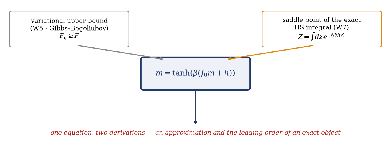
So the same equation now has two derivations, and Figure 13.2 records the fork. From the left, mean field is a variational upper bound: the exact functional evaluated on a restricted family, with the one-sided guarantee \(F_q \geq F\) of Equation 9.1. From the right, it is a saddle point: the leading order of an exact integral, with no guarantee but with a systematic sequence of corrections attached. The two views are complementary in precisely the way Week 6 needed: it is because mean field is the leading order of something exact that its corrections (the fluctuations the bound discards) are computable rather than mysterious.

Figure 13.2: Two derivations, one equation. Week 5 reached \(m = \tanh(\beta(J_0 m + h))\) by restricting the variational family and minimizing the Gibbs–Bogoliubov bound; today reaches it as the stationary point of the exact Hubbard–Stratonovich integral. The bound explains why mean field is an approximation with a guaranteed sign; the saddle explains why it is the leading order of a systematic expansion, with corrections that are the auxiliary field’s fluctuations.

Corrections are the field’s fluctuations. Laplace’s method carries its own error estimate, and here the error has a name. Expanding \(f\) to second order around the saddle and using Equation 2.2, the prefactors combine into

\[ Z \;\approx\; e^{-N \beta f(z^{*})}\, \sqrt{\frac{J}{f''(z^{*})}}, \qquad f''(z^{*}) \;=\; J \big[ 1 - \beta J (1 - z^{*2}) \big] \;=\; \frac{\beta J (1 - z^{*2})}{\chi}, \]

where \(\chi = \partial m / \partial h\) is the susceptibility of the model, obtained by differentiating Equation 13.3. The Gaussian width of the auxiliary field around its saddle is therefore set by \(1/f''\) — by the susceptibility. Far from the transition, \(f''\) is of order one, the field barely fluctuates, and the corrections to mean field are \(\mathcal{O}(1/N)\); as \(T \to T_c\) the susceptibility diverges (the Curie–Weiss law of Section 10.3), \(f''(z^*) \to 0\), the integrand flattens, and the fluctuations of the auxiliary field grow without bound. This is Week 5’s audit and Week 6’s correction program, re-derived from one integral: mean field is exact when the field cannot fluctuate — the fully connected model as \(N \to \infty\), where the saddle is infinitely sharp — and fails where the field fluctuates strongly, near criticality. What the variational route called “discarded correlations” the saddle route calls “fluctuations of \(z\)”: the same physics, carried by \(f''\).

Take-home 2

Evaluating the exact integral Equation 13.2 by Laplace’s method gives \(z^* = \tanh(\beta(Jz^* + h))\) — Week 5’s mean-field equation, with \(z^*\) equal to the magnetization and \(f(z^*)\) equal to the variational free energy at its optimum. Mean field is the saddle point of an exact representation; its corrections are the Gaussian fluctuations of the auxiliary field, of size \(1/f''(z^*) \propto \chi\) — small at \(\mathcal{O}(1/N)\) generically, divergent at the critical point.

13.4 The auxiliary field is a latent variable

Everything so far evaluated the integral. The reframe that closes Module 2 comes from refusing to: instead of integrating over \(z\), read the integrand of Equation 13.2 as a probability distribution. The object under the integral, before the spin sum is performed, is a perfectly well-formed joint distribution over the spins and the field together,

\[ p(s, z) \;=\; \frac{1}{Z} \sqrt{\frac{N \beta J}{2\pi}}\; \exp\!\Big[ -\frac{N \beta J}{2} z^{2} + \beta (J z + h) \sum_i s_i \Big], \]

whose marginal over \(z\) is, by construction, exactly the Curie–Weiss Boltzmann distribution — that is what Equation 13.2 asserts. Now factor this joint the other way. Conditioned on \(z\), the spins are independent, each governed by the normalized single-site factor

\[ p(s_i \mid z) \;=\; \frac{e^{\beta (J z + h) s_i}}{2 \cosh(\beta (J z + h))} \;=\; \sigma\!\big( 2 \beta (J z + h)\, s_i \big), \]

a sigmoid \(\sigma(u) = 1/(1 + e^{-u})\) in the field — the logistic unit of every neural network, appearing here as the exact conditional of a spin given the auxiliary field. (The symbol \(\sigma\) is the logistic function throughout this lecture, unrelated to the encoder standard deviation \(\sigma_\phi\) of the next lecture’s VAE.) And the marginal of the field itself, obtained by summing the joint over the spins, is \(p(z) \propto e^{-N \beta f(z)}\): the very integrand whose saddle we just took, now in the role of a prior over \(z\). Assembling the two factors,

\[ \boxed{\; p(s) \;=\; \int \mathrm{d}z\; p(z) \prod_i p(s_i \mid z), \qquad p(z) \propto e^{-N \beta f(z)}, \qquad p(s_i \mid z) = \sigma\big(2\beta (Jz + h)\, s_i\big) \;} \tag{13.4}\]

the latent-variable reframe

This is a latent-variable generative model, and it is the Curie–Weiss ferromagnet with no approximation: draw a field \(z\) from its prior, then draw each spin independently from a sigmoid conditioned on \(z\). The recipe even samples correctly through the phase transition — below \(T_c\) the prior \(e^{-N\beta f(z)}\) concentrates on the two wells \(\pm m\) of Section 10.3, so drawing \(z\) first amounts to choosing a symmetry-broken branch, after which the spins fall independently in line. The interaction has become a hidden common cause: spins look correlated to anyone who cannot see \(z\), and become independent the moment \(z\) is revealed. The star graph of Figure 13.1 was the claim; Equation 13.4 is the proof. (A bookkeeping remark for the careful reader: one may equally keep the bare Gaussian weight \(e^{-N\beta J z^2/2}\) as the prior, at the price of unnormalized conditionals — normalizing the sigmoids is what moves the factor \([2\cosh]^N\) into \(p(z)\). Both factorizations describe the same joint; Equation 13.4 is the one in which every factor is a distribution.)

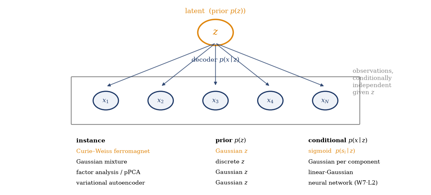
The general model. Strip the physics and the structure that remains is \[ p(x) \;=\; \int \mathrm{d}z\; p(z)\, p(x \mid z), \] a prior over a hidden variable and a conditional — machine learning calls it the decoder — over the observations. This one template covers a remarkable fraction of generative modeling (Figure 13.3): a Gaussian mixture is a discrete \(z\) with one Gaussian per component; factor analysis and probabilistic PCA are a Gaussian \(z\) with a linear-Gaussian decoder; the variational autoencoder of the next lecture (Kingma and Welling 2014) is a Gaussian \(z\) with a neural-network decoder. The instances differ only in the two distributions plugged into the template; the conditional-independence structure — the star — is common to all of them. And the physics supplies what the template alone does not: an answer to where the latent comes from and how many dimensions it should have. The eigendecomposition remark of Section 13.2 says that a general interaction \(J = \sum_\mu \lambda_\mu v_\mu v_\mu^{\mathsf T}\) decouples into one field per eigenvalue: the latent dimension counts the independent modes of the interaction. Curie–Weiss is rank one and needs a single latent; data whose correlations have many strong modes need as many decoupling fields — which is, from this shore, why the latent spaces of real generative models are high-dimensional.

Figure 13.3: One structure, many models. The latent-variable graphical model — a hidden \(z\) with conditionally independent observations \(x_1, \ldots, x_N\) — realized by different choices of prior and conditional. The Curie–Weiss ferromagnet, decoupled by Hubbard–Stratonovich, is an exact instance with a one-dimensional latent; the variational autoencoder (the next lecture) is the same structure with a neural decoder.

The solvable instance: a linear-Gaussian decoder. One member of the zoo is worked out in full, because it is the only one whose inference problem closes in a formula — and because it turns the eigenmode count above into numbers (Welling, Lu, and Holdijk 2026, ch. 4 on latent-variable models). Take a Gaussian latent and a linear decoder with isotropic noise,

\[ p(z) = \mathcal{N}(0, \mathbb{1}_K), \qquad p(x \mid z) = \mathcal{N}(W z,\, \sigma^2 \mathbb{1}), \]

so that a sample is assembled as \(x = W z + \sigma\, \varepsilon\): \(K\) hidden modes, mixed by the columns of \(W\), plus noise — factor analysis with equal noise variances, better known as probabilistic PCA (Tipping and Bishop 1999). Everything the general template leaves intractable is here explicit. The joint log-density is quadratic in \(z\), so the posterior is Gaussian and completing the square — the same move that proved Equation 13.1 — is the entire computation:

\[ \log p(z \mid x) \;=\; -\frac{1}{2\sigma^2} \| x - W z \|^2 - \frac{1}{2} \|z\|^2 + \text{const} \;=\; -\frac{1}{2}\, z^{\mathsf{T}} \Big( \mathbb{1} + \frac{W^{\mathsf{T}} W}{\sigma^2} \Big) z + \frac{1}{\sigma^2}\, z^{\mathsf{T}} W^{\mathsf{T}} x + \text{const}, \]

whence

\[ p(z \mid x) = \mathcal{N}\big( \mu(x),\, C \big), \qquad C = \Big( \mathbb{1} + \frac{W^{\mathsf{T}} W}{\sigma^2} \Big)^{-1}, \qquad \mu(x) = \frac{1}{\sigma^2}\, C\, W^{\mathsf{T}} x . \]

the one closed-form posterior in the zoo

(The evidence follows just as cheaply: \(x\) is a linear map of jointly Gaussian variables, so \(p(x) = \mathcal{N}(0,\, W W^{\mathsf{T}} + \sigma^2 \mathbb{1})\) — the marginal likelihood, in closed form, for this one model.) Read the posterior along the decoder’s own axes and the eigenmode claim becomes quantitative. Take the columns of \(W\) orthogonal, \(W_\mu = w_\mu u_\mu\) with orthonormal \(u_\mu\): then \(W^{\mathsf{T}} W\) is diagonal, the posterior factorizes over modes, and each latent coordinate is a shrunken projection of the data onto its mode,

\[ \mu_\mu(x) \;=\; \frac{w_\mu^2}{w_\mu^2 + \sigma^2}\; \frac{u_\mu^{\mathsf{T}} x}{w_\mu}, \qquad C_{\mu\mu} \;=\; \frac{\sigma^2}{w_\mu^2 + \sigma^2} . \]

The bracket in front is a per-mode signal-to-noise weight: a strong mode (\(w_\mu^2 \gg \sigma^2\)) is read off the data essentially verbatim, while a weak one (\(w_\mu^2 \ll \sigma^2\)) is shrunk toward the prior’s zero, its posterior variance staying close to the prior’s one — the inference is effectively suppressed where noise dominates. The claim of Section 13.2 — that the latent dimension counts the interaction’s strong eigenmodes — is here a formula rather than a principle. The instance matters for the module because of what happens when it breaks: replace \(W z\) by a neural network and both closed forms vanish, since no conjugacy survives the first nonlinearity. That loss is exactly the intractability the next lecture’s encoder is trained to patch — the VAE’s variational posterior \(q_\phi(z \mid x) = \mathcal{N}(\mu_\phi(x), \sigma_\phi(x))\) keeps the shape of the formula above and learns the map \(x \mapsto (\mu, \sigma)\) that the linear model derives.

Learning the model, and the loop back to Week 5. The physics handed us \(p(z)\) and \(p(x \mid z)\) complete, because we knew the Hamiltonian. Machine learning faces the inverse task: given samples of \(x\) and a parameterized decoder \(p_\theta(x \mid z)\), fit \(\theta\) by maximizing the evidence \(\log p_\theta(x) = \log \int \mathrm{d}z\, p(z)\, p_\theta(x \mid z)\) — and both the integral and the posterior \(p(z \mid x)\) it hides are intractable, for the same reason \(Z\) always was. The resolution is the one this module has rehearsed since Week 5: maximize a lower bound, the ELBO, which Equation 9.2 identified as minus the variational free energy, with the posterior gap \(D_\mathrm{KL}(q(z) \| p(z \mid x))\) as the exact deficit. The classical algorithm built on this bound is EM (Dempster, Laird, and Rubin 1977): the E-step sets \(q\) to the current posterior (closing the gap), the M-step maximizes \(\langle \log p_\theta(x, z) \rangle_q\) over \(\theta\) (raising the bound) — coordinate ascent on the ELBO, forty years before that name existed. What the next lecture adds is scale: when the posterior is not computable even per data point, a neural encoder learns to approximate it for all \(x\) at once, and the result is the variational autoencoder. The physics that creates latent variables (Hubbard–Stratonovich) and the inference that learns them (the ELBO) are now both on the table; only the neural realization remains.

Trap

The auxiliary field is not physical — but its saddle is. Under the integral, \(z\) ranges over all real values and carries no physical meaning; attributing reality to its fluctuating value is a category error. Only the saddle \(z^*\) equals the magnetization, and only as \(N \to \infty\). Two corollaries follow. ① Mean field is the saddle, not the integral: equating them silently drops the fluctuation corrections, which is precisely the error Weeks 5–6 spent two lectures diagnosing. ② The transformation’s simple real form needs a positive-definite interaction; applying Equation 13.1 blindly to a coupling with negative eigenvalues produces a divergent Gaussian — those modes need imaginary fields, and the bookkeeping is not optional.

Take-home 3

Read rather than evaluated, the Hubbard–Stratonovich integrand is a latent-variable model: \(p(s) = \int \mathrm{d}z\, p(z) \prod_i p(s_i \mid z)\), with the integrand-as-prior \(p(z) \propto e^{-N\beta f(z)}\) and sigmoid conditionals — the Curie–Weiss ferromagnet exactly. The general template \(p(x) = \int \mathrm{d}z\, p(z)\, p(x \mid z)\) covers mixtures, factor analysis, and the VAE; the latent dimension counts the interaction’s eigenmodes; and learning the model is Week 5’s ELBO again, with EM as its classical coordinate ascent.

13.5 Example: the saddle against the truth

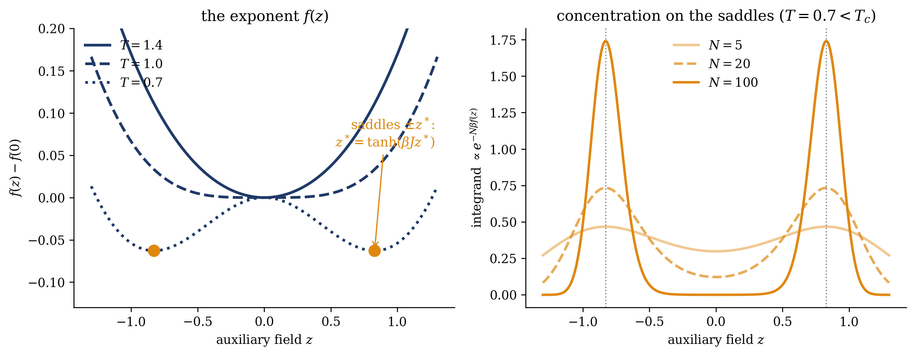
The two claims — the integral is exact, and mean field is only its saddle — can be tested against each other on one small model. Take Curie–Weiss at \(J = 1\) (so \(T_c = 1\)), \(h = 0\), and \(T = 0.7\), comfortably in the ordered phase. The saddle equation Equation 13.3 gives \(z^* = 0.8286\) with \(f(z^*) = -0.5480\) and curvature \(f''(z^*) = 0.552\); the exact free energy per spin comes from the magnetization-sector sum of Section 10.5, affordable at any \(N\). Figure 13.4 draws the two halves of the story: the exponent \(f(z)\) developing the double well of Section 10.3 as \(T\) crosses \(T_c\) — the same landscape, now living on the auxiliary field — and the integrand \(e^{-N\beta f(z)}\) sharpening onto the saddles as \(N\) grows.

\(N\)	\(f_\text{exact}\)	\(f_\text{saddle}\)	gap	saddle + fluctuation	residual
\(5\)	\(-0.6819\)	\(-0.5480\)	\(0.134\)	\(-0.6866\)	\(0.0047\)
\(20\)	\(-0.5859\)	\(-0.5480\)	\(0.038\)	\(-0.5827\)	\(0.0032\)
\(100\)	\(-0.5551\)	\(-0.5480\)	\(0.0070\)	\(-0.5550\)	\(0.0001\)
\(1000\)	\(-0.54872\)	\(-0.54802\)	\(0.00069\)	\(-0.54871\)	\(5 \times 10^{-6}\)

The columns confirm the analysis. The gap column shrinks in proportion to \(1/N\) — tenfold between \(N = 100\) and \(N = 1000\): the saddle approximation converges to the truth as \(1/N\), which is the precise sense in which mean field is exact for the fully connected model — the verdict of Section 10.4, now visible inside a single integral. The last two columns identify the gap completely: adding the Gaussian-fluctuation prefactor of Section 13.3, together with a factor of \(2\) because both wells contribute below \(T_c\), predicts the free energy as \(f(z^*) - \frac{T}{N} \ln\!\big( 2 \sqrt{J / f''(z^*)} \big)\), and this lands within \(10^{-4}\) of the exact answer already at \(N = 100\). The correction to mean field is the width of the peak (and the number of peaks), and the formula is known — the same lesson Section 2.6 taught for Stirling’s series, returning at the end of the module.

Show code

from scipy.special import gammaln

J = 1.0  # T_c = J = 1

def f(z, T):
    return 0.5 * J * z**2 - T * np.log(2 * np.cosh(J * z / T))

def saddle(T):
    z = 0.9
    for _ in range(20000):
        z = np.tanh(J * z / T)
    return z

fig, (a1, a2) = plt.subplots(1, 2, figsize=(10.4, 4.1))
zz = np.linspace(-1.3, 1.3, 600)
for T, ls in zip([1.4, 1.0, 0.7], ["-", "--", ":"]):
    a1.plot(zz, f(zz, T) - f(0.0, T), color=NAVY, ls=ls, lw=2.2, label=rf"$T = {T}$")
zst = saddle(0.7)
a1.plot([zst, -zst], [f(zst, 0.7) - f(0, 0.7)] * 2, "o", color=ORANGE, ms=9, zorder=5)
a1.annotate(r"saddles $\pm z^*$:" "\n" r"$z^*=\tanh(\beta J z^*)$",
            xy=(zst, f(zst, 0.7) - f(0, 0.7)), xytext=(1.28, 0.06),
            ha="right", color=ORANGE, fontsize=10.5,
            arrowprops=dict(arrowstyle="->", color=ORANGE, lw=1))
a1.set_xlabel(r"auxiliary field $z$")
a1.set_ylabel(r"$f(z) - f(0)$")
a1.set_title(r"the exponent $f(z)$", fontsize=12)
a1.legend(frameon=False, fontsize=10, loc="upper left")
a1.set_ylim(-0.13, 0.2)

T = 0.7
for N, ls, al in zip([5, 20, 100], ["-", "--", "-"], [0.45, 0.7, 1.0]):
    g = np.exp(-N / T * (f(zz, T) - f(zst, T)))
    g /= g.sum() * (zz[1] - zz[0])  # normalize on the grid
    a2.plot(zz, g, color=ORANGE, ls=ls, lw=2.0, alpha=al, label=rf"$N = {N}$")
a2.axvline(zst, color=GRAY, ls=":", lw=1)
a2.axvline(-zst, color=GRAY, ls=":", lw=1)
a2.set_xlabel(r"auxiliary field $z$")
a2.set_ylabel(r"integrand $\propto e^{-N\beta f(z)}$")
a2.set_title(rf"concentration on the saddles ($T = {T} < T_c$)", fontsize=12)
a2.legend(frameon=False, fontsize=10, loc="upper center")
fig.tight_layout()
plt.show()

Figure 13.4: The exact partition function as one integral, concentrating on mean field (\(J = 1\), \(h = 0\), so \(T_c = 1\)). Left: the exponent \(f(z)\) of Equation 13.2 at three temperatures, drawn relative to \(f(0)\) — a single well at \(z = 0\) above \(T_c\), a flattening at \(T_c\), and the double well of Section 10.3 below it, now as a function of the auxiliary field; the orange dots mark the saddles \(\pm z^*\) from Equation 13.3 (\(z^* = 0.83\) at \(T = 0.7\)). Right: the normalized integrand \(e^{-N\beta f(z)}\) at \(T = 0.7\) for growing \(N\) — the weight concentrates onto the saddles, with width shrinking as \(1/\sqrt{N \beta f''(z^*)}\), and Laplace’s method Equation 2.2 becomes exact. Mean field is the \(N \to \infty\) limit of this picture; everything it misses is the remaining width.

One consistency check ties the module together. The double well in the left panel of Figure 13.4 and the double well of Figure 10.2 are drawn from different functions — Week 5’s landscape lives on the trial magnetization, today’s on the auxiliary field — yet their minima sit at the same \(\pm m\) with the same depth, as Section 13.3 proved they must. The phase transition of Section 10.2 can therefore be read a third way: it is the moment the exact integrand of \(Z\) changes from one peak to two, and spontaneous symmetry breaking is the statement that as \(N \to \infty\) the integral is captured entirely by whichever peak the field \(h \to 0^+\) selects.

A latent variable is a decoupling field — a generative model is an interacting system with the interaction integrated out.

The week continues from here. The evening before the next lecture: the warm-up card, on the ELBO and reparameterization sections of the VAE review by Kingma and Welling (2019) — every object in that paper now has a physical name: the prior is a decoupling field’s distribution, the decoder is the conditional the field induces, and the training objective is Week 5’s variational free energy with its sign flipped. In the next lecture the model becomes trainable: neural encoder and decoder, the reparameterization trick that makes the latent integral differentiable, and the variational autoencoder in full (Kingma and Welling 2014). The tutorial is computation-led, training a VAE on MNIST and decomposing its ELBO term by term.

13.6 Outlook: Module 2 closes

Module 2 set out to tame one intractable object, the interacting Boltzmann distribution, and it left four methods on the table. Week 5 bounded it: the Gibbs–Bogoliubov inequality on a factorized family, with the ELBO as its inference-side name. Week 6 corrected the bound (the reaction term of Chapter 11) and then reorganized it into messages on the interaction graph (Chapter 12). Today transformed it: the interaction removed exactly, the system rewritten as a latent-variable generative model, and mean field re-derived as the saddle of the exact representation. The unifying object throughout has been a single functional — the variational free energy, equal to minus the ELBO by Equation 9.2 — optimized over different families, corrected by different terms, and returning in the next lecture as the training loss of the variational autoencoder. A 1950s identity from quantum field theory (Stratonovich 1957; Hubbard 1959) and the objective of a 2014 deep generative model (Kingma and Welling 2014) belong to the same three-week story.

A broader principle generalizes beyond the ferromagnet: wherever a latent-variable model fits data well, an interacting system stands behind it, with the latent as its decoupling field and the latent’s typical values as its order parameters. The correlations in data play the role the interaction played here; the latent dimensions count its strong eigenmodes; and inference over the latent is the physics of a field near its saddle. Machine learning rediscovered this structure independently, because marginalizing a shared cause and decoupling an interaction are the same mathematical act read in opposite directions.

Every method of this module — bound, correction, messages, transformation — manipulated the form of the distribution without visiting its configurations. Module 3, beginning in Week 8, takes the complementary approach and samples: Monte Carlo and the Metropolis rule, simulated annealing, and the Langevin dynamics whose stationary measure is the Boltzmann distribution itself — the machinery that will let us treat stochastic gradient descent as a finite-temperature physical process. The distribution approximated over three weeks will now be sampled directly.