Core (~1 h).Jaynes (1957), §§1–4 — the origin of the maximum-entropy argument we carry out below: inference as the least-committal distribution consistent with what is known. This is the single source the lecture is built on. Alongside it, the introduction and §II of Mehta et al. (2019), which set up the physics↔︎ML vocabulary — energy, loss, likelihood — that the whole course speaks; this review is also the reference text for the tutorials.
Optional background. The probability-and-entropy chapters of Schwarz (2023), for anyone who wants their master’s statistical mechanics refreshed to the level this course assumes; MacKay (2003), Ch. 2–4, for entropy and inference from the information-theory side; Sethna (2021), Ch. 5–6, for entropy and free energy with the “thinking in probabilities” emphasis we lean on. The historical anchors — Shannon (1948), Hopfield (1982), Ackley, Hinton, and Sejnowski (1985) — return as primary sources in Weeks 2–3, so a first pass now pays off later.
Prerequisite reminder. The Boltzmann distribution, entropy, and free energy are assumed from master’s statistical mechanics. From the companion Machine Learning and Physics course we assume only fluency with the softmax layer, which the identification in §The softmax is a Boltzmann distribution rests on; a reader arriving without it should read Mehta et al. (2019) §II first. What is new here is the framing of these objects as the shared substrate of generative machine learning — not the objects themselves.
1.1 Why a nineteenth-century equation keeps reappearing
We write three objects side by side. The Boltzmann distribution of statistical mechanics,
\[
p(x) \propto e^{-\beta E(x)},
\]
the softmax layer that terminates essentially every classifier trained today,
\[
p_i = \frac{e^{z_i}}{\sum_j e^{z_j}},
\]
and the score of a probability distribution,
\[
\nabla_x \log p(x),
\]
the vector field a diffusion model learns in order to turn noise into images. The first two are the same equation; the third is that equation differentiated, which is precisely what removes the normalizer, since for \(p \propto e^{-\beta E}\) the score is \(-\beta \nabla_x E\) — the force of the energy landscape, with \(Z\) gone. The resemblance is not an analogy but a pedigree. By the end of this lecture we will have proven that the first two are identical; Week 10 establishes the third, and Week 12 identifies the score with the noise-prediction target \(\varepsilon_\theta\) that industrial diffusion models actually minimize.
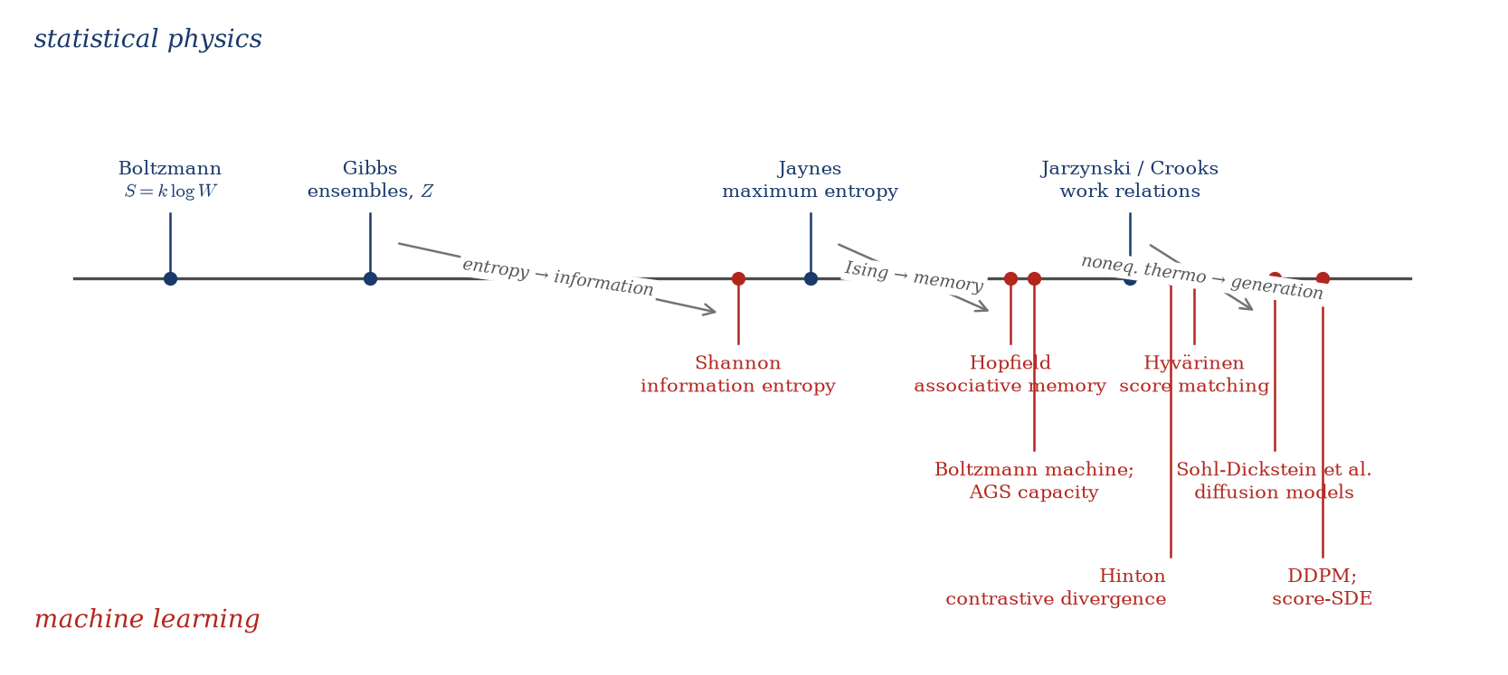
The claim rests on a precise intellectual lineage, traced in Figure 1.1, in which physics and what we now call machine learning have exchanged the same mathematical object for a century and a half. Boltzmann gave entropy a statistical meaning in the 1870s — \(S = k \log W\), the equation on his tombstone in Vienna (the constant-bearing form is Planck’s): entropy counts the microstates consistent with a macrostate, and probability enters physics. Gibbs (1902) systematized the idea into ensembles and the canonical distribution \(p \propto e^{-\beta E}\), together with its normalizer, the partition function\(Z\) — from the German Zustandssumme, “sum over states.” The object this whole course revolves around is already on the page in 1902.
The pivot comes at mid-century. Shannon (1948) defined the information entropy \(H = -\sum_i p_i \log p_i\) — the same functional Gibbs wrote down, but now measuring uncertainty in a message rather than heat in a gas. Jaynes (1957) then turned the logic around: the equilibrium distribution of statistical mechanics is nothing but the maximum-entropy distribution consistent with what one knows, so that the usual computational rules of the field, beginning with the determination of the partition function, “are an immediate consequence of the maximum-entropy principle.” With Jaynes, the Boltzmann distribution stops being a statement about molecules and becomes a principle of inference — and inference is what learning machines do. This is the derivation we carry out in full in Section 1.4.
The machine-learning lane takes over in 1982. Hopfield (1982) imported the Ising energy function into computer science: a recurrent network of binary units whose dynamics roll downhill on an energy landscape, with memories stored as its minima — learning becomes the shaping of a landscape. Ackley, Hinton, and Sejnowski (1985) made the construction stochastic and trainable, the Boltzmann machine, and immediately hit the wall this course is organized around: the training gradient requires an expectation under the model, and that expectation requires \(Z\). Amit, Gutfreund, and Sompolinsky (1985) answered a quantitative question with spin-glass methods — how many patterns can a Hopfield network store? — obtaining the celebrated capacity \(\alpha_c \approx 0.138\) patterns per neuron (Amit, Gutfreund, and Sompolinsky 1987), the first time the statistical mechanics of disordered systems yielded a quantitative, closed-form theory of a learning system. Hinton (2002) supplied a practical dodge: contrastive divergence approximates the intractable model expectation with a short Gibbs chain — cheap, biased, and enormously influential.
The modern turn reunites the two lanes. Hyvärinen (2005) showed that an unnormalized model can be fit by matching the score\(\nabla_x \log p\), in which \(Z\) drops out entirely because \(\nabla_x \log Z = 0\) — the clean elimination, where before there had only been evasions. In parallel, nonequilibrium statistical mechanics produced the work relations of Jarzynski (1997) and Crooks (1999), which recover equilibrium free-energy differences — ratios of partition functions — from finite-time, driven trajectories. Sohl-Dickstein et al. (2015) read that literature and built a generative model from it explicitly: destroy structure with a forward diffusion, learn the reverse process, and generation is nonequilibrium thermodynamics run backwards. Denoising diffusion probabilistic models (Ho, Jain, and Abbeel 2020) made the construction state of the art, and Song et al. (2021) unified the whole family as a forward stochastic differential equation plus a reverse-time SDE driven by the score \(\nabla_x \log p_t\). Every reappearance in this story is the same normalization, met and evaded in a new form.
The mathematics of counting configurations weighted by energy is the same mathematics whether the configurations are gas microstates, stored memories, or images — and the recurring hard part is always the same normalization.
This also fixes the course’s position relative to its companion. Machine Learning and Physics teaches the working methods — how to run a DDPM, a VAE, an MCMC chain. This course is its structural-derivation complement: we derive why those methods work, from statistical mechanics — reverse-time SDEs, the Jarzynski and Crooks relations, the Fokker–Planck equation of training, mean-field and replica theory.
Figure 1.1: The pedigree this course traces. Two lanes — statistical physics above the axis, machine learning below — keep handing the same object back and forth: Gibbs’s partition function becomes Shannon’s entropy, Jaynes’s inference principle, Hopfield’s landscape, the Boltzmann machine’s training obstruction, and finally the diffusion model’s generative engine. Gray arrows mark the crossings.
Take-home 1
Statistical physics and generative machine learning are two dialects of one language: probability distributions defined by an energy. This course traces the derivation, not the analogy.
1.2 The bridge, in two directions
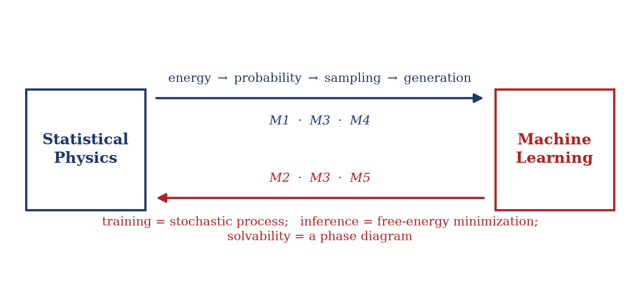
The traffic across this bridge runs both ways; the two directions organize all fourteen weeks (Figure 1.2).
In the physics → ML direction, an energy function defines a probability distribution; learning becomes shaping an energy landscape so that the data sit in its basins, and generation becomes sampling from the shaped landscape. Modules 1, 3 and 4 live on this arrow. In the ML → physics direction, the tools of statistical mechanics are turned onto learning itself: training under stochastic gradients is a stochastic process with its own Fokker–Planck equation and stationary measure, and inference is variational free-energy minimization. Modules 2 and 3 live on this arrow, and so does Module 5, aimed at a different target: Modules 2 and 3 turn the machinery on learning algorithms and ask what a given method computes and how accurately, while Module 5 turns it on learning problems and asks which of them admit a solution at all. Week 13’s detectability threshold is a statement about a task, not about any particular method for it.
Figure 1.2: The two-way bridge, and the filing cabinet for the semester. Physics → ML: an energy defines a probability, learning shapes the landscape, generation samples it (Modules 1, 3, 4). ML → physics: training is a stochastic process, inference is free-energy minimization, and solvability itself has a phase diagram (Modules 2, 3, 5).
Beneath both directions sits one operational tension that every week of the course responds to: for essentially every interesting model, the unnormalized weight \(e^{-E(x)}\) is trivial to write down and to evaluate at any single configuration — while its normalizer
\[
Z = \sum_x e^{-E(x)}
\]
is intractable. Everything hard in this course is a strategy for living with, approximating, or eliminating \(Z\).
The course map follows directly. We open with the shared foundations (this week). Module 1 (Weeks 2–4) develops the energy-based view — Hopfield networks, Boltzmann machines and contrastive divergence, modern energy-based models, and the identification of modern Hopfield networks with attention — and it is here that \(Z\) is raised as the training obstruction. Module 2 (Weeks 5–7) develops the variational and mean-field toolbox — the variational free energy, TAP equations, belief propagation and approximate message passing, Hubbard–Stratonovich transformations and variational autoencoders — where \(Z\) is approximated. Module 3 (Weeks 8–9) treats sampling and the Fokker–Planck equation of training — Markov chain Monte Carlo, Langevin dynamics, simulated annealing, SGD-as-Langevin and flat minima — where \(Z\) is sampled around. Module 4 (Weeks 10–12) is the resolution: the nonequilibrium thermodynamics of generative modeling — score matching, the Jarzynski and Crooks relations, annealed importance sampling, DDPM and score-based SDEs — where \(Z\) is eliminated. Module 5 (Week 13) turns the same machinery on representation and on inference itself: the information bottleneck, where \(Z\) normalizes an encoder and compression is traded against relevance at an inverse temperature, and the phase transitions of statistical inference, where a partition function over hypotheses decides which problems are solvable at all. Week 14 synthesizes.
The course’s spine — and the backbone of the exam — runs from Week 3, “the Boltzmann machine cannot be trained because \(\nabla_\theta \log Z\) is intractable,” to Week 10, “score matching removes \(Z\) because \(\nabla_x \log Z = 0\).” Note the subscripts: the obstruction is a gradient with respect to the parameters\(\theta\); the escape is a gradient with respect to the configuration\(x\). These are different derivatives of the same offending object, and the precision matters — we return to it in Week 10.
Take-home 2
You can always write the model down; you can almost never normalize it. The partition function \(Z\) is the through-line of the course — raised as an obstruction in Module 1, resolved in Module 4.
1.3 The shared vocabulary
Students arrive here with statistical mechanics already in hand, so we do not re-derive; we state and cite, and use the space for the machine-learning reframing. The following panel fixes the notation for all fourteen weeks.
Symbol
Meaning
Notes
\(x\)
configuration / microstate
a gas microstate, a spin configuration, a stored pattern, an image — deliberately overloaded
\(E(x)\)
energy / cost
physics Hamiltonian \(=\) ML loss, score, negative log-likelihood
\(\beta\)
inverse temperature \(1/T\)
clashes with ML’s \(\beta\) (e.g. \(\beta\)-VAE, Adam’s \(\beta_{1,2}\)) — we always mean \(1/T\)
\(Z\)
partition function\(\sum_x e^{-\beta E(x)}\)
the course’s through-line
\(F\)
(Helmholtz) free energy\(-T \log Z\)
\(= \langle E \rangle - TS\)
\(S\)
entropy \(-\sum_x p(x) \log p(x)\)
a functional of a distribution, not of one state
\(\langle \cdot \rangle\)
expectation
subscript the distribution: \(\langle \cdot \rangle_\text{data}\), \(\langle \cdot \rangle_\text{model}\)
\(p(x),\ q(x)\)
model / variational (or data) distributions
fixed per lecture
\(\theta\)
model parameters
gradients \(\nabla_\theta\)
\(\nabla_x\)
gradient w.r.t. the configuration
distinct from \(\nabla_\theta\) — the score-matching distinction hinges on this
We fix three conventions once and use them throughout. First, we set \(k_B = 1\): temperature is measured in energy units and entropy is dimensionless. Second, \(\log\) means the natural logarithm throughout, so entropy is measured in nats — with that choice the information-theoretic and thermodynamic entropies are literally the same object, not proportional ones; where a base-2 aside is needed we will write \(\log_2\) explicitly. Third, energies always enter as \(e^{-\beta E}\): lower energy means higher probability, and on the ML side the logits will accordingly be negative energies.
Two of the entries in the panel call for a comment. The energy \(E(x)\) is, in physics, a Hamiltonian one measures; in machine learning it is a loss or score one designs — same mathematical role, opposite provenance, and the whole of Module 1 lives in that shift. The free energy \(F = -T \log Z = \langle E \rangle - TS\) is the logarithm of the very object we cannot compute; when Module 2 constructs variational bounds, it is \(F\) they bound.
Trap
Entropy in this course is a functional of a distribution, not a property of a single configuration. A configuration has an energy; only an ensemble has an entropy. Students arriving from a thermodynamics-first background routinely conflate the two; keep them separate.
1.4 Maximum entropy and the Boltzmann distribution
We now carry out the derivation in full. The question it answers is an inference question, and posing it that way is Jaynes’s insight (Jaynes 1957).
Suppose we have an energy function \(E(x)\) over configurations, and suppose the only thing we know about the system is its average energy \(\langle E \rangle = U\). What probability distribution \(p(x)\) should we assign? We refuse to smuggle in any assumption beyond what we actually know — and that refusal can be formalized: among all distributions consistent with the constraints, choose the one of maximum entropy,
\[
S[p] = -\sum_x p(x) \log p(x),
\]
because any distribution of lower entropy encodes information we do not possess. The constraints are ① normalization, \(\sum_x p(x) = 1\), and ② the known mean energy, \(\sum_x p(x)\, E(x) = U\).
The derivation. We maximize \(S[p]\) subject to ① and ② with Lagrange multipliers \(\alpha\) and \(\beta\):
The underbraced prefactor carries no \(x\)-dependence; it is fixed entirely by normalization ①. Imposing it defines the normalizer the whole course revolves around,
⇒ The maximum-entropy distribution consistent with a known mean energy is exponential in the energy — nothing else is assumed.
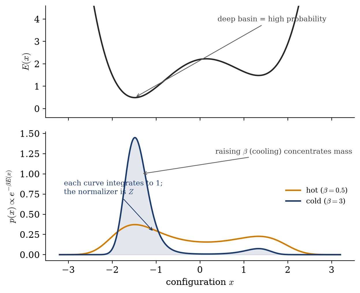
What is \(\beta\)? Mechanically, it is the multiplier that enforces the energy constraint, tuned so that \(\langle E \rangle = U\); physically, we identify it as the inverse temperature, \(\beta = 1/T\). The two limits make the identification vivid, and Figure 1.3 draws them: at low \(\beta\) (hot), the exponential is nearly flat and probability spreads almost uniformly over configurations; at high \(\beta\) (cold), the mass collapses onto the ground state — the global minimum of the landscape. In one line: temperature is the exchange rate between entropy and energy. An ML reader already knows this dial — it is the “temperature” setting on a language model’s sampler, and it is the same \(\beta\).
Figure 1.3: The central picture of the course. Top: an energy landscape \(E(x)\) with basins of unequal depth. Bottom: the Boltzmann densities \(p(x) \propto e^{-\beta E(x)}\) it induces at \(\beta = 0.5\) (hot — nearly flat) and \(\beta = 3\) (cold — mass concentrated in the deep basin). Each curve integrates to one, and the normalizer that enforces this is \(Z\); temperature tunes exploration against exploitation.
A second lens. There is more in the same result. \(Z(\beta)\) is not merely a normalizer; it is a generating function. Differentiating \(\log Z\) produces the observables: \(\langle E \rangle = -\partial \log Z / \partial \beta\), and the second derivative gives the energy fluctuations and hence the heat capacity (both derived in the next lecture, in Chapter 2, and they return quantitatively in Module 5). Knowing \(Z\) is knowing everything about the equilibrium ensemble — which is exactly why its intractability is so costly.
Trap
\(Z\) is not a constant you may ignore. Change any parameter of \(E\) and \(Z\) changes with it; in a learned model, \(\nabla_\theta \log Z\) is exactly the term that blocks training. The habit of “dropping the normalization” — harmless in a homework problem — is a reflex to unlearn before this course.
1.5 The softmax is a Boltzmann distribution
The corollary takes four lines. Let the configurations be class labels, \(x \in \{1, \dots, K\}\), and let a network’s last layer output the logits \(z_1, \dots, z_K\). Define the energy of class \(i\) to be \(E_i = -z_i\) and set \(\beta = 1\). Then Equation 1.2 reads
⇒ The softmax layer is a Boltzmann distribution over labels, and its denominator is a partition function over \(K\) states.
Every reader of these notes has been computing partition functions daily, under an assumed name. The reason \(Z\) has never hurt: a classifier sums over \(K \approx 10\)–\(10^3\) classes, and a sum with a thousand terms is free. The moment the configurations are not labels but high-dimensional objects — images, spin configurations, molecules — the same sum acquires exponentially many terms, and the field’s difficulty begins. The next section makes that quantitative.
Two further identifications are flagged now and derived later. The cross-entropy loss is \(-\log p_\text{correct}\) — a free-energy difference — and minimizing it is maximum-likelihood estimation on a Boltzmann model (shown in Week 3). And the relation between \(F\), the Kullback–Leibler divergence, and variational bounds is the engine of Module 2. Neither is derived today.
1.6 Example: two states, then the \(2^N\) wall
A toy that works. Take the smallest possible system: one binary unit, \(x \in \{0, 1\}\), with \(E(0) = 0\) and \(E(1) = \Delta E > 0\), so that state 0 is the ground state. The partition function has exactly two terms, \(Z = 1 + e^{-\beta \Delta E}\), and the occupation of the excited state is
Measuring temperature in units of the gap, \(\tau \equiv T/\Delta E\), the numbers behave as follows:
\(\beta \Delta E\)
\(\tau = T/\Delta E\)
\(p(1)\)
reading
\(0\)
\(\infty\)
\(0.500\)
hot: both states equally likely
\(\ln 2 \approx 0.693\)
\(1.44\)
\(0.333\)
excited : ground \(= 1 : 2\)
\(1\)
\(1.00\)
\(0.269\)
thermal energy equals the gap
\(2\)
\(0.50\)
\(0.119\)
—
\(5\)
\(0.20\)
\(0.0067\)
cold: mass collapses onto the ground state
\(\to \infty\)
\(\to 0\)
\(\to 0\)
only the ground state survives
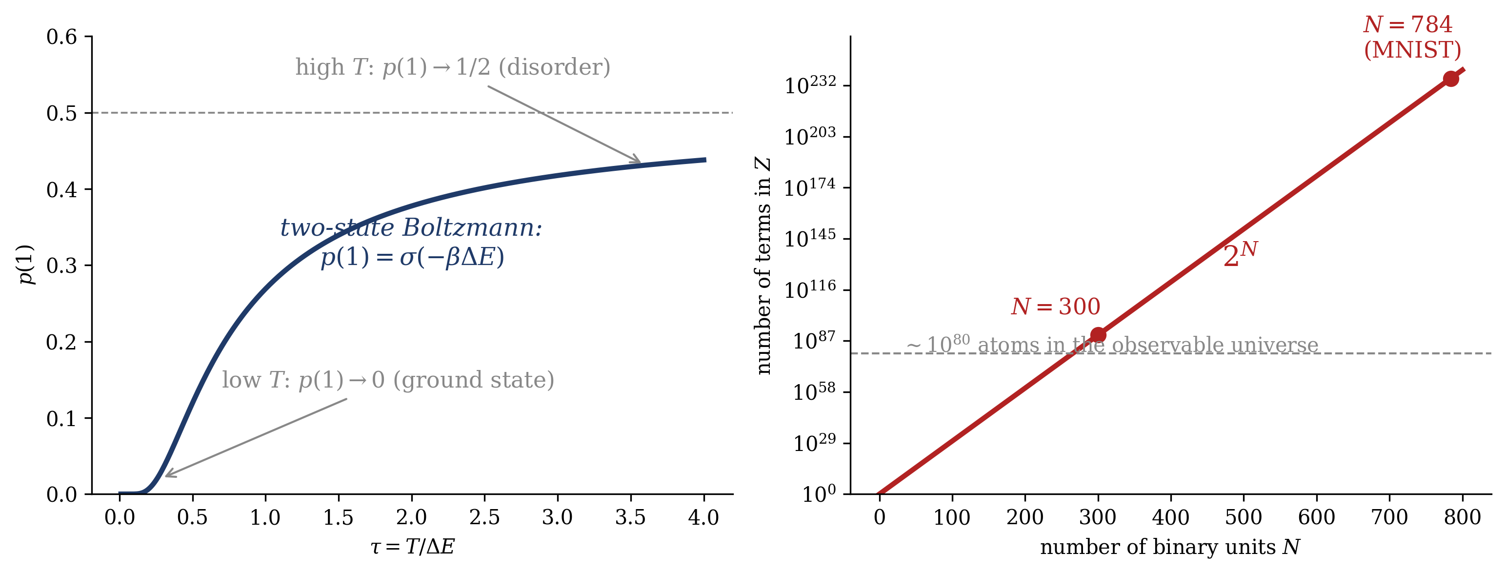
As a function of the gap at fixed temperature, the same occupation reads \(p(1) = \sigma(-\beta \Delta E)\) with \(\sigma(u) = 1/(1 + e^{-u})\) — the logistic function. The sigmoid of every neural-network textbook is the two-state Boltzmann distribution, the second such identification of the day. The left panel of Figure 1.4 draws the occupation against temperature instead, reading off the two limits of the table.
The wall. Now let the system grow: \(N\) binary units — an Ising layer, or the visible layer of a small restricted Boltzmann machine. The partition function
\[
Z = \sum_{x \in \{0,1\}^N} e^{-\beta E(x)}
\]
has \(2^N\) terms, and the right panel of Figure 1.4 shows what that exponential means in practice. For \(N = 10\), \(Z\) has \(1{,}024\) terms — trivial. For \(N = 300\), it has \(2^{300} \approx 2 \times 10^{90}\) terms, roughly ten orders of magnitude more than the \(\sim 10^{80}\) atoms in the observable universe. For \(N = 784\) — the pixels of one small MNIST image — it has \(2^{784} \approx 10^{236}\).
An order-of-magnitude check makes the cost concrete. Grant an optimistic \(10^9\) energy evaluations per second. Brute-forcing the \(N = 300\) partition function then takes \(\sim 10^{90}/10^9 = 10^{81}\) seconds, against a universe whose age is \(\approx 4.4 \times 10^{17}\) seconds — about \(10^{63}\) ages of the universe for one number. And yet evaluating \(e^{-\beta E(x)}\) at any single configuration costs a microsecond.
Figure 1.4: Left: the excited-state occupation \(p(1)\) of the two-state system (\(E(0)=0\), \(E(1)=\Delta E\)) against reduced temperature \(\tau = T/\Delta E\), with \(p(1) \to 1/2\) at high temperature and \(p(1) \to 0\) as the mass collapses onto the ground state; as a function of the gap at fixed temperature, the same occupation is the logistic \(\sigma(-\beta\Delta E)\). Right: the number of terms in \(Z\), equal to \(2^N\), against the number of binary units \(N\); the dashed line marks the \(\sim 10^{80}\) atoms in the observable universe, crossed already at \(N \approx 266\), with \(N = 300\) and \(N = 784\) (one MNIST image) indicated.
Evaluating one configuration is free; summing over all of them is impossible — and that single asymmetry is why Modules 1–4 exist. You can always write the model down; you can almost never normalize it.
In the Week 3 tutorial you will hit this \(2^N\) wall yourselves, on a real Boltzmann machine. The resolution comes in Week 10.
Take-home 3
The cost of \(Z\) is exponential in system size: computable for a softmax over \(K\) labels, hopeless for a distribution over configurations. The entire course is strategies for that gap.
Trap
“Softmax has no partition-function problem” is true only because \(K\) is small. The same object over configurations — not labels — is intractable. Do not let the benign case set your intuition for the general one.
1.7 Course mechanics and the contract
The practical arrangements are stated once, here, and kept current on the course-information page. Fourteen weeks, five modules, two 90-minute lectures per week (Lectures 1 and 2, 9–11) plus an afternoon tutorial (16–18); 8 credit points. The grade is a written final exam, 100% — no graded problem sets. The exam is built directly from the tutorials’ in-class problems and is organized along the \(Z\) spine, so preparing for the exam is doing the tutorials; it is closed-book, and any formula the exam needs but does not expect you to memorize is provided on the paper. Exam admission is an ungraded Studienleistung: submit the weekly stuck-point card for at least 8 of the 12 tutorial warm-ups, which run from Week 2.
The tutorials run every week and follow a productive-failure format: a light warm-up at home (a short reading and a small priming task, whose stuck-point card feeds the session’s triage), then the hard problem — revealed only in the room and cracked in groups. Come having attempted the crux; meeting the wall in class is part of the design. On the weeks whose problem is computational, bring a laptop if you have one: after a silent individual attempt and a written group prediction, each group opens one machine for about twenty minutes and fills in a small number of marked lines in a prepared notebook, and the closing round runs on the projector for the room. One machine per group of three or four is enough, so not everyone needs to carry one. On the weeks whose problem is a derivation there are no machines at all. The exam tests computational reasoning rather than live coding.
This course does not develop rigorous large-deviation theory, does not give the renormalization group its full due, and does not treat the hardware and systems side of machine learning; each would be its own course, and the reading list points to where they are done well. What this course does claim is the derivational road set out at the start of this chapter: not how to run the methods, but why they work — with the partition function as the recurring obstruction.
1.8 Outlook
The next lecture assembles the quantitative foundations we lean on all semester: ensembles, the free-energy identities used as working tools rather than slogans, maximum entropy as an inference engine, and the Gaussian and saddle-point machinery that recurs from Module 2 onward. Week 2 then opens Module 1 with the Hopfield model — the Ising energy repurposed as an associative memory, and the first time in the course that \(E(x)\) is something we design rather than measure.
All three take-home points reduce to one: you can always write the model down; you can almost never normalize it.
Ackley, David H., Geoffrey E. Hinton, and Terrence J. Sejnowski. 1985. “A Learning Algorithm for Boltzmann Machines.”Cognitive Science 9 (1): 147–69. https://doi.org/10.1207/s15516709cog0901_7.
Amit, Daniel J., Hanoch Gutfreund, and Haim Sompolinsky. 1985. “Storing Infinite Numbers of Patterns in a Spin-Glass Model of Neural Networks.”Physical Review Letters 55 (14): 1530–33. https://doi.org/10.1103/PhysRevLett.55.1530.
Crooks, Gavin E. 1999. “Entropy Production Fluctuation Theorem and the Nonequilibrium Work Relation for Free Energy Differences.”Physical Review E 60 (3): 2721–26. https://doi.org/10.1103/PhysRevE.60.2721.
Gibbs, J. Willard. 1902. Elementary Principles in Statistical Mechanics. New Haven: Yale University Press.
Hinton, Geoffrey E. 2002. “Training Products of Experts by Minimizing Contrastive Divergence.”Neural Computation 14 (8): 1771–1800. https://doi.org/10.1162/089976602760128018.
Ho, Jonathan, Ajay Jain, and Pieter Abbeel. 2020. “Denoising Diffusion Probabilistic Models.” In Advances in Neural Information Processing Systems. Vol. 33. https://arxiv.org/abs/2006.11239.
Hopfield, John J. 1982. “Neural Networks and Physical Systems with Emergent Collective Computational Abilities.”Proceedings of the National Academy of Sciences 79 (8): 2554–58. https://doi.org/10.1073/pnas.79.8.2554.
Hyvärinen, Aapo. 2005. “Estimation of Non-Normalized Statistical Models by Score Matching.”Journal of Machine Learning Research 6: 695–709.
MacKay, David J. C. 2003. Information Theory, Inference, and Learning Algorithms. Cambridge: Cambridge University Press.
Mehta, Pankaj, Marin Bukov, Ching-Hao Wang, Alexandre G. R. Day, Clint Richardson, Charles K. Fisher, and David J. Schwab. 2019. “A High-Bias, Low-Variance Introduction to Machine Learning for Physicists.”Physics Reports 810: 1–124. https://doi.org/10.1016/j.physrep.2019.03.001.
Sohl-Dickstein, Jascha, Eric Weiss, Niru Maheswaranathan, and Surya Ganguli. 2015. “Deep Unsupervised Learning Using Nonequilibrium Thermodynamics.” In Proceedings of the 32nd International Conference on Machine Learning, 37:2256–65. Proceedings of Machine Learning Research. https://arxiv.org/abs/1503.03585.
Song, Yang, Jascha Sohl-Dickstein, Diederik P. Kingma, Abhishek Kumar, Stefano Ermon, and Ben Poole. 2021. “Score-Based Generative Modeling Through Stochastic Differential Equations.” In International Conference on Learning Representations. https://arxiv.org/abs/2011.13456.