Core (~1 h).Thouless, Anderson, and Palmer (1977) — six pages, and the best-titled paper in this syllabus: the corrected mean-field theory of the Sherrington–Kirkpatrick model, containing the reaction term this lecture derives; read for the equations and for the quotation marks in the title. Alongside it, re-read Mézard and Montanari (2009), Ch. 2, whose cavity formulation our physical route follows. (The belief-propagation chapter, ch. 14, is the next lecture’s warm-up pre-read — the keen may start it early, but stop before the messages become algorithms.)
Optional background.Plefka (1982) — the systematic expansion behind the engine, naive mean field and TAP as its first two orders; Georges and Yedidia (1991) — the expansion continued, every higher correction generated mechanically; Onsager (1936) — the original reaction field, in dielectrics, sixty years before machine learning rediscovered it; Mézard, Parisi, and Virasoro (1987) — the cavity method and the many-states picture, for depth; Opper and Saad (2001) for TAP in inference.
Prerequisite reminder. All of Week 5 — the variational bound and its ELBO reading, the factorized ansatz and Equation 9.3, the audit and its verdict — plus Week 2’s disordered couplings (Hebb, the AGS feedback factor \(r\)) and one fact from Week 1’s two-state spin that we will re-derive in a line: its susceptibility. New content: the reaction/cavity argument, the Plefka expansion, the TAP equations, the \(\sum_j J_{ij}^2\) scaling analysis, and the estimate-versus-bound trade.
11.1 The debt, and a pointed title
Last week’s audit ended in a verdict — mean field discards every correlation, over-predicts order, and where it fails is where variational inference needs corrections — and the tutorial made the gap visible on a projector. Today we begin the correction. Naive mean field will turn out to be the first order of a controlled expansion, its leading correction is a single term with a crisp physical meaning, and the size of that term will tell us — quantitatively, model by model — when Week 5’s theory was trustworthy and when it was quietly wrong.
The history behind that term frames the whole of Module 2, and it runs through Week 2’s own lineage. In 1975, Sherrington and Kirkpatrick proposed a mean-field spin glass — Gaussian random couplings, every spin coupled to every other — and, with disarming confidence, titled the paper Solvable Model of a Spin-Glass(Sherrington and Kirkpatrick 1975). They then solved it, by the replica method, and their solution carried a defect they themselves flagged: at low temperature the entropy goes negative — for discrete spins, an impossibility, the thermodynamic equivalent of a proof ending in \(1 = 2\). Two years later, Thouless, Anderson, and Palmer published the corrected mean-field theory under the title Solution of “Solvable Model of a Spin Glass”(Thouless, Anderson, and Palmer 1977) — the quotation marks serving as a referee report. Their correction to the mean-field equations is one term. Today we earn it, twice: once by a short physical argument, and once by an expansion that tells us exactly what order of what series the argument computed. (The SK saga’s full resolution — Parisi’s replica symmetry breaking, and a 2021 Nobel prize — is a mountain this course walks beside rather than over; the outlook says precisely how our road relates to it.)
The driving question: what is the first correction to mean field, and when is it large? The correction is subtracting your own echo — removing from each spin’s effective field the part that the spin itself put there, reflected back by its neighbors. And its size is governed by \(\sum_j J_{ij}^2\): of order \(1/N\) for the uniform ferromagnet Week 5 audited — invisible, which is why naive mean field passed that audit — but of order one for disordered couplings, which is to say for the SK model, for Week 2’s Hebb-built networks, and for essentially every model whose couplings were written by data rather than by symmetry.
Take-home 1
Naive mean field is not a dead end but the first order of a systematic expansion. Its leading correction — the Onsager reaction term, Thouless, Anderson, and Palmer (1977) — subtracts from each spin’s field the part that spin itself put there. The correction is \(\mathcal{O}(1/N)\) for uniform dense couplings and \(\mathcal{O}(1)\) for disordered ones: the models that matter live on the corrected side.
11.2 The echo: the field you feel versus the field you cause
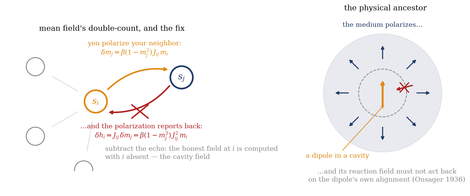
The physical argument first, because it fits in a picture that carries the central idea. The naive effective field of Equation 9.3, \(\sum_j J_{ij} m_j + h_i\), treats each neighbor’s magnetization as independent evidence about what spin \(i\) should do. But look at where \(m_j\) comes from: \(j\) sits, in part, in the field of \(i\) itself. Spin \(i\) polarizes its neighbor through the bond; the polarized neighbor reports back through the same bond; and the naive field counts that report as one more vote for what \(i\) already is. A consistent theory must not let a spin respond to its own echo.
One line of Week 1 makes the echo quantitative. A single spin in a field \(h\) has \(m = \tanh(\beta h)\), so its susceptibility — its readiness to respond — is
an undecided spin (\(m_j \approx 0\)) responds maximally; a saturated one (\(m_j \to \pm 1\)) barely responds at all. That is the only new ingredient the correction needs, and it is not new. Assemble the echo (Figure 11.1): spin \(i\) shifts its neighbor by \(\delta m_j = \chi_j J_{ij} m_i\); the shifted neighbor feeds back the field \(\delta h_i = J_{ij}\, \delta m_j = \beta (1 - m_j^2)\, J_{ij}^2\, m_i\). Note the square of the coupling — echoes travel out along the bond and back along the same bond, so they always carry \(J^2\). Summing over neighbors and subtracting gives the corrected field:
the cavity field: \(i\)’s field with \(i\)’s own influence removed
— the cavity field, so called because it is the field at site \(i\) computed as if \(i\) sat in a cavity: the neighbors’ magnetizations taken as they would be in \(i\)’s absence. (Conceptually, the correct inputs are the cavity magnetizations \(m_j^{(i)}\) — \(j\)’s value with \(i\) removed — and the reaction term is exactly the bookkeeping that converts the full \(m_j\) into them, to the order computed: \(m_j = m_j^{(i)} + \chi_j J_{ij} m_i + \mathcal{O}(J^3)\). That distinction matters loosely today and exactly in the next lecture, because keeping “who was removed” straight is precisely what message passing does.) The idea is much older than spin glasses: Onsager (1936) introduced the reaction field for dielectrics — a molecular dipole polarizes the liquid around it, and the returning polarization field must not be counted when computing the dipole’s own alignment (Figure 11.1, right). TAP’s move was to import a forty-year-old piece of electrostatics into disordered magnetism; ours, this week, is to import it into inference.
Figure 11.1: The central picture of the lecture. Left: mean field’s double-count — spin \(i\) polarizes its neighbor \(j\) by \(\delta m_j = \beta(1-m_j^2)J_{ij}m_i\) (orange), and the polarization reports back as a field \(\propto J_{ij}^2 m_i\) (red, struck out): a spin’s own influence, returning as fake evidence. Subtracting the echo yields the cavity fieldEquation 11.1 — the field at \(i\) computed with \(i\) absent. Right: the physical ancestor (Onsager 1936) — a dipole polarizes the surrounding medium, and the medium’s reaction field must not act back on the dipole’s own alignment.
Writing \(m_i = \tanh(\beta h_i^\text{cav})\) already gives the corrected self-consistency — the TAP equations, in fact. But at this point they are physics, not yet a controlled approximation: we do not know what the argument neglected, what “order” it computed, or how to go further. The Plefka expansion answers all three.
11.3 The engine: the Plefka expansion
Setup. We want an expansion whose zeroth order is free spins, whose knob is the interaction strength, and whose variables are the magnetizations — so that each order corrects the theory of \(m\), not just the free energy. The right object is the constrained (Gibbs) free energy \(G(\lambda, m)\): the free energy of the Hamiltonian with its exchange part scaled by an interpolation parameter \(\lambda \in [0,1]\) (\(J \to \lambda J\); the external fields ride along unscaled), evaluated with the magnetizations pinned to prescribed values \(m_i\). The pinning is done by auxiliary Lagrange fields \(b_i\) adjusted at every \(\lambda\) so that \(\langle s_i \rangle = m_i\) exactly — the Legendre-transform bookkeeping is spelled out in Plefka (1982) and Georges and Yedidia (1991), and the script keeps only what the board needs: at \(\lambda = 0\) the constrained measure factorizes, so every average is computable, and derivatives of \(G\) in \(\lambda\) are averages of the interaction in that computable ensemble. Expand around \(\lambda = 0\), then set \(\lambda = 1\). (One notational flag: the literature writes this parameter \(\alpha\); we rename it \(\lambda\) because \(\alpha\) is this course’s storage load, and that collision is not worth carrying.)
Order zero — independent spins. At \(\lambda = 0\), pinned free spins are Week 5’s factorized ansatz exactly, and \(G\) is pure entropy: \(\beta G_0 = -\sum_i S(m_i)\), the binary entropy per site, minus the field term \(\beta \sum_i h_i m_i\).
Order one — Week 5, recovered. The first derivative is the average of the exchange energy in the factorized reference, where \(\langle s_i s_j \rangle = m_i m_j\):
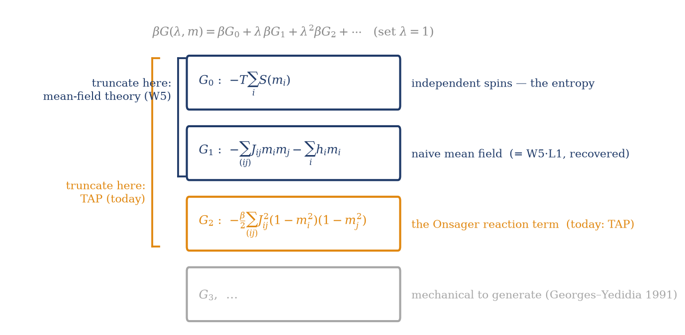
Assemble \(G_0 + \lambda G_1\) at \(\lambda = 1\) and you are holding, symbol for symbol, Week 5’s mean-field free energy. This reframes the whole of last week: naive mean field is the first-order truncation of this expansion. It was never an isolated ansatz; it was rung one of a ladder (Figure 11.2), and the ladder continues.
Order two — the Onsager term, derived. The second derivative of \(G\) in \(\lambda\) is (minus \(\beta\) times) a variance: the fluctuation of the exchange energy about its mean, in the constrained reference. Two lines of moment algebra do the evaluation. The fluctuating object is \(\sum_{(ij)} J_{ij}(s_i s_j - m_i m_j)\); squaring and averaging over independent spins, distinct bonds decorrelate, and each bond contributes \(\langle (s_i s_j)^2 \rangle - \cdots = 1 - m_i^2 m_j^2\) — from which the constraint (the \(b_i\) readjusting at each order so the magnetizations stay pinned) removes the pieces where only one spin of the bond fluctuates, \(m_j^2(1 - m_i^2) + m_i^2(1 - m_j^2)\), leaving exactly
per bond: the product of the two ends’ single-site variances — that is, of their susceptibilities, the very objects that carried the echo. The second-order term is therefore \(G_2 = -\tfrac{\beta}{2} \sum_{(ij)} J_{ij}^2 (1-m_i^2)(1-m_j^2)\), and truncating the ladder here gives the TAP free energy:
Stationarity gives the equations. Differentiate in \(m_i\): the naive part gives Week 5’s terms (\(-h_i^\text{eff}\) from the energy, \(T\operatorname{artanh}(m_i)\) from the entropy), and the new term contributes \(+\beta\, m_i \sum_j J_{ij}^2 (1 - m_j^2)\). Setting the sum to zero and inverting:
— the TAP equations(Thouless, Anderson, and Palmer 1977): Week 5’s self-consistency with one new term inside the \(\tanh\), and that term is precisely the echo of Equation 11.1. The two derivations serve different purposes: the physical route says why (a spin must not respond to its own reflection), the expansion says what (second order in the coupling) and what next (the third and higher rungs are generated mechanically — Georges and Yedidia (1991) give the algorithm, and nothing but patience stands between you and \(G_3\)).
Figure 11.2: The engine’s map: mean field is not a guess but a truncation. The constrained free energy expands in the interaction strength as \(\beta G = \beta G_0 + \lambda\,\beta G_1 + \lambda^2 \beta G_2 + \cdots\): order zero is the entropy of pinned free spins, order one is Week 5’s mean-field theory — recovered, not assumed — and order two is the Onsager reaction term, whose per-bond weight \((1-m_i^2)(1-m_j^2)\) is the product of the two ends’ susceptibilities. Truncate after \(G_1\) and you hold W5·L1; truncate after \(G_2\) and you hold TAP; the ladder continues mechanically (Georges and Yedidia 1991).
Take-home 2
The Plefka expansion of the fixed-\(m\) free energy in the coupling: order one is Week 5’s mean field; order two adds \(-\tfrac{\beta}{2}\sum J_{ij}^2(1-m_i^2)(1-m_j^2)\), whose stationarity gives the TAP equations — the effective field minus the spin’s own echo, reflected through \(J_{ij}^2\) and weighted by the neighbors’ susceptibilities. Higher orders are mechanical.
11.4 When the echo matters — and what TAP costs
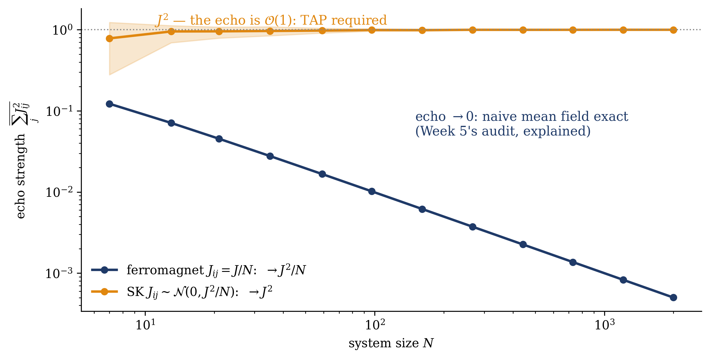
The scaling verdict. The reaction term rides on one number, \(\sum_j J_{ij}^2\), and its value across coupling ensembles is the central scaling result (Figure 11.3):
Uniform ferromagnet, \(J_{ij} = J/N\):\(\sum_j J_{ij}^2 = J^2 (N-1)/N^2 \to 0\). The echo vanishes in the thermodynamic limit — and Week 5’s audit, which found naive mean field exact on precisely this model, is now explained rather than observed. Nothing was lucky about it: the model’s couplings are individually so weak that no spin meaningfully polarizes any neighbor.
SK disorder, \(J_{ij} \sim \mathcal{N}(0, J^2/N)\):\(\sum_j J_{ij}^2 \to J^2\) by the law of large numbers — order one, at every temperature. Individual couplings are strong enough (\(\sim 1/\sqrt{N}\)) to polarize neighbors, and the echoes, though random in sign as fields, add their squares. For disordered couplings the reaction term is not a refinement; it is the difference between a wrong theory and a usable one — which is why SK’s “solvable” model needed TAP. On the SK model the term takes a famously compact form: \(\sum_j J_{ij}^2 (1 - m_j^2) \to J^2 (1 - q)\) with \(q = \frac{1}{N}\sum_j m_j^2\) — the Edwards–Anderson overlap, Week 2’s \(q\), returning to the course in its home country.
The same physics appeared in Week 2, without its name. The AGS retrieval theory’s noise-amplification factor \(r = (1-C)^{-2}\) in Equation 4.5 — the term that moved the capacity from \(2/\pi\) to \(0.138\) — is the network responding to its own errors: flipped bits polarize the fields that flipped them. That was a reaction effect, quoted as a result then, derived as a principle now. Hebb couplings at extensive load are exactly the disordered, \(\mathcal{O}(1)\)-echo kind — learning writes disordered couplings, so the models this course cares about live generically on the corrected side of the verdict.
Figure 11.3: The scaling verdict, sampled: the echo’s driver \(\frac{1}{N}\sum_i \sum_j J_{ij}^2\) against system size for the two coupling ensembles (20 instances per size; bands span the instances). For the uniform ferromagnet \(J_{ij} = J/N\) (navy) the sum decays as \(J^2/N\) — the reaction term vanishes in the thermodynamic limit, which is why Week 5’s audit found naive mean field exact on exactly this model. For SK disorder \(J_{ij} \sim \mathcal{N}(0, J^2/N)\) (orange) it converges to \(J^2\): order one at every size and every temperature. One number decides who needs TAP — and learned, data-built couplings are of the disordered kind.
What was traded. Week 5’s one-sided guarantee does not survive the correction. \(F_q \geq F\) held because \(F_q\) was the exact variational functional evaluated on a restricted family. \(F_\text{TAP}\) is a truncated expansion — the exact functional of no family at all — and the guarantee does not survive truncation: \(F_\text{TAP}\) is generally much closer to the truth and can sit on either side of it (in the example below it sits below the exact \(F\) at every temperature shown). This is a real loss, and it recurs across the course’s methods: contrastive divergence traded unbiasedness for tractability (Week 3); TAP trades the bound for accuracy. Each successive method in the course gains precision at the expense of formal guarantees. (The next lecture partially restores the variational character at the pairwise level, via the Bethe free energy; the loss is specific to the Plefka truncation, not to the correction program.)
Many solutions, and trouble iterating. A further cost is physical rather than formal. At high temperature the TAP equations have one solution; lower the temperature into the glass region of a disordered model and they develop many — exponentially many for SK — each a metastable valley of the corrected free-energy landscape, the many states of Mézard, Parisi, and Virasoro (1987). This is Week 2’s ruggedness surfacing inside a deterministic approximation, and it has an inference-side reading Week 5 prepared: multiple TAP solutions are multiple local optima of a corrected ELBO-like objective — the two ferromagnetic wells of last week, multiplied by disorder into a landscape. Practical corollary: naive fixed-point iteration of Equation 11.3 can oscillate or diverge exactly where the physics is interesting (our example uses damping), and the iteration whose error can be tracked exactly, step by step, arrives in the next lecture under an algorithm’s name.
The ML echo. The same machinery runs inference in learning systems directly: Kappen and Rodríguez (1998) showed that a Boltzmann machine’s intractable statistics — Week 3’s negative phase \(\langle s_i s_j \rangle_\text{model}\) — can be estimated deterministically by solving the TAP equations and reading correlations from linear response, replacing the sampling chains of contrastive divergence with a corrected mean-field computation. The correction term remains a working component of inverse-Ising and Boltzmann-machine inference.
Trap
“Second order” does not mean small — and \(F_\text{TAP}\) is not a bound. ① For disordered couplings the second-order term is \(\mathcal{O}(1)\) — the same size as the first — at every temperature; order in the expansion is position on a ladder, not magnitude, and the magnitude is set by \(\sum_j J_{ij}^2\) alone. ② Truncating the ladder destroys Week 5’s one-sidedness: \(F_\text{TAP}\) can dip below the true \(F\) and promises no error sign. Bound versus estimate — always know which you are holding, and never report a TAP solution as the solution inside the glass phase, where there are exponentially many.
Take-home 3
The echo’s size is \(\sum_j J_{ij}^2\): vanishing for the uniform ferromagnet (\(J^2/N\) — Week 5’s exactness, explained), order one for SK-type disorder (\(J^2(1-q)\), with Week 2’s Edwards–Anderson \(q\) returning) — and learning writes disordered couplings. The price of the correction: the bound is gone (TAP is an estimate — the CD trade again), and inside the glass phase the equations have exponentially many solutions with real convergence trouble for naive iteration.
11.5 Example: one term, from wrong to right
One disordered instance, small enough to enumerate, so that every claim can be checked directly. Take \(N = 10\) spins with SK couplings \(J_{ij} \sim \mathcal{N}(0, J^2/N)\), \(J = 1\), and small random fields (\(h_i \sim \mathcal{N}(0, 0.2^2)\), to break the global flip symmetry); \(2^{10} = 1024\) states gives the exact \(F\) and \(\langle s_i \rangle\) by brute force. Solve Week 5’s naive equations and today’s TAP equations by damped iteration from the same start, and compare — the same three-column protocol as Week 5’s example, now with disorder doing the judging:
\(T\)
RMS error, naive MF
RMS error, TAP
\(F_\text{exact}\)
\(F_\text{naive}\)
\(F_\text{TAP}\)
\(2.0\)
\(0.051\)
\(0.009\)
\(-15.06\)
\(-14.01\)
\(-15.15\)
\(1.5\)
\(0.227\)
\(0.027\)
\(-11.96\)
\(-10.69\)
\(-12.10\)
\(1.2\)
\(0.419\)
\(0.064\)
\(-10.22\)
\(-9.01\)
\(-10.43\)
\(0.8\)
\(0.460\)
\(0.225\)
\(-8.19\)
\(-7.49\)
\(-8.65\)
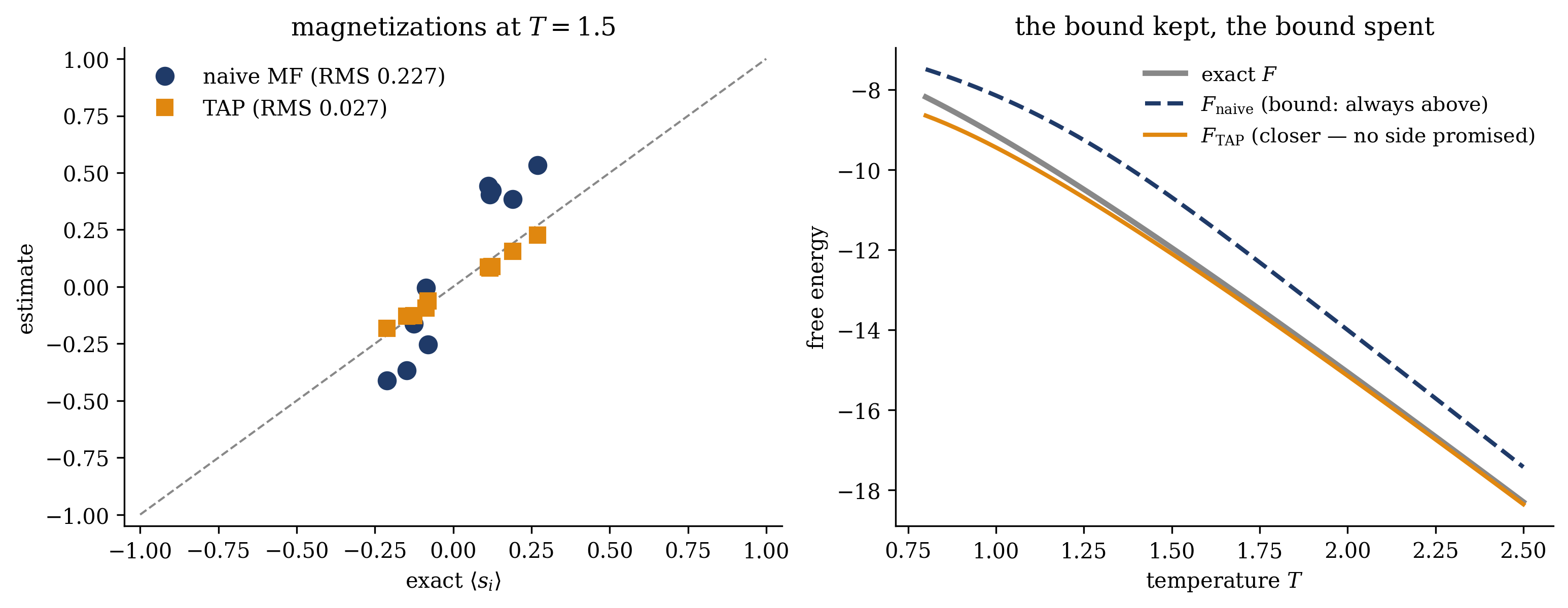
The columns track the predictions above. The error columns are the headline: at \(T = 1.5\) the single reaction term cuts the magnetization error eightfold (\(0.227 \to 0.027\)); at \(T = 1.2\), sixfold. One term takes the theory from wrong to right, on a model whose \(\sum_j J_{ij}^2\) is order one — exactly as the verdict predicts. The free-energy columns show both costs at once: \(F_\text{naive}\) sits above the truth at every temperature (Week 5’s bound, holding faithfully — off by \(1.3\) at \(T = 1.5\)), while \(F_\text{TAP}\) sits far closer (\(0.15\) at \(T = 1.5\)) but below the truth — the lost bound, visible directly. And the last row makes the third cost numerical: at \(T = 0.8\), inside the glass phase of this model, TAP’s own error grows to \(0.23\) — the territory of many solutions and higher-order physics, where no truncation of the ladder is safe and the next lecture’s algorithmic ideas become necessary. Figure 11.4 draws the \(T = 1.5\) magnetizations and the free-energy curves. For contrast, run the same pipeline on the uniform ferromagnet (\(J_{ij} = J/N\), same \(N\)): the naive and TAP magnetizations agree to \(0.03\) — a gap that is pure \(1/N\), shrinking with size — and the echo term is invisible, as the verdict says it must be.
Show code
def make_sk(N, J, seed): rng = np.random.default_rng(seed) Jm = rng.normal(0, J / np.sqrt(N), (N, N)) Jm = (Jm + Jm.T) / np.sqrt(2) np.fill_diagonal(Jm, 0.0) h = rng.normal(0, 0.2, N)return Jm, hdef exact(Jm, h, T): N =len(h) S = np.array([[(c >> i &1) *2-1for i inrange(N)] for c inrange(2**N)], dtype=float) E =-0.5* np.einsum("ci,ij,cj->c", S, Jm, S) - S @ h w = np.exp(-(E - E.min()) / T) p = w / w.sum()return-T * np.log(w.sum()) + E.min(), (p[:, None] * S).sum(axis=0)def solve(Jm, h, T, tap, damp, iters=20000, tol=1e-12): m = np.full(len(h), 0.01) J2 = Jm**2for _ inrange(iters): field = Jm @ m + hif tap: field = field - (1/ T) * m * (J2 @ (1- m**2)) # the reaction term m_new = np.tanh(field / T)if np.abs(m_new - m).max() < tol:return m_new m = (1- damp) * m + damp * m_newreturn mdef free_energies(Jm, h, T, m, tap): S_ent = np.sum(-(1+ m) /2* np.log((1+ m) /2) - (1- m) /2* np.log((1- m) /2)) F =-0.5* m @ Jm @ m - h @ m - T * S_entif tap: F -= (1/ (2* T)) * np.sum(np.triu(Jm**2, 1) * np.outer(1- m**2, 1- m**2))return FN =10Jm, h = make_sk(N, 1.0, seed=8)fig, (a1, a2) = plt.subplots(1, 2, figsize=(10.4, 4.1))T0 =1.5_, mex = exact(Jm, h, T0)mmf = solve(Jm, h, T0, tap=False, damp=0.5)mtap = solve(Jm, h, T0, tap=True, damp=0.3)a1.plot([-1, 1], [-1, 1], color=GRAY, ls="--", lw=1)a1.plot(mex, mmf, "o", color=NAVY, ms=8, label=rf"naive MF (RMS {np.sqrt(np.mean((mmf-mex)**2)):.3f})")a1.plot(mex, mtap, "s", color=ORANGE, ms=7, label=rf"TAP (RMS {np.sqrt(np.mean((mtap-mex)**2)):.3f})")a1.set_xlabel(r"exact $\langle s_i \rangle$"); a1.set_ylabel("estimate")a1.set_title(rf"magnetizations at $T = {T0}$", fontsize=12)a1.legend(frameon=False, fontsize=10, loc="upper left")a1.set_xlim(-1.05, 1.05); a1.set_ylim(-1.05, 1.05)Ts = np.linspace(0.8, 2.5, 60)Fex, Fmf, Ftap = [], [], []for T in Ts: F, _ = exact(Jm, h, T) m1 = solve(Jm, h, T, tap=False, damp=0.5) m2 = solve(Jm, h, T, tap=True, damp=0.3) Fex.append(F) Fmf.append(free_energies(Jm, h, T, m1, tap=False)) Ftap.append(free_energies(Jm, h, T, m2, tap=True))a2.plot(Ts, Fex, color=GRAY, lw=2.6, label=r"exact $F$")a2.plot(Ts, Fmf, color=NAVY, ls="--", lw=2.0, label=r"$F_\mathrm{naive}$ (bound: always above)")a2.plot(Ts, Ftap, color=ORANGE, lw=2.0, label=r"$F_\mathrm{TAP}$ (closer — no side promised)")a2.set_xlabel(r"temperature $T$"); a2.set_ylabel("free energy")a2.set_title("the bound kept, the bound spent", fontsize=12)a2.legend(frameon=False, fontsize=9.5, loc="upper right")fig.tight_layout(); plt.show()
Figure 11.4: The correction at work, on an enumerable SK instance (\(N = 10\), \(J_{ij} \sim \mathcal{N}(0, 1/N)\), small random fields; exact values from all \(1024\) states). Left: per-spin magnetizations at \(T = 1.5\), estimate against truth — naive mean field (navy) scatters off the diagonal (RMS error \(0.227\)); adding the one reaction term (TAP, orange) collapses the points onto it (RMS \(0.027\)). Right: free energies across temperature. \(F_\mathrm{naive}\) (navy dashed) sits above the exact \(F\) everywhere — Week 5’s variational bound, intact. \(F_\mathrm{TAP}\) (orange) hugs the truth an order of magnitude closer — and from below: the truncated expansion keeps no side of the truth, the guarantee spent for the accuracy. Inside the glass phase (left edge) all truncations degrade — the many-states territory.
A spin must not respond to its own echo — subtracting the echo is the entire first correction to mean field, and on disordered couplings the echo is \(\mathcal{O}(1)\).
The week continues from here. The evening before the next lecture: the warm-up card, on the belief-propagation introduction of Mézard and Montanari (2009), ch. 14 — the cavity field derived above is the object that chapter passes along the edges of a graph. In the next lecture, the cavity goes onto a sparse graph and becomes an algorithm with a variational functional of its own; the tutorial is derivation-led, deriving that algorithm at the board alongside its modern descendant from signal processing.
11.6 Outlook: from cavity to messages
Module 2’s program now stands as follows. The variational road now has two stations: the bound (Week 5 — exact functional, restricted family, guaranteed sign) and the correction (today — truncated expansion, better numbers, no sign), with the ladder above them mechanical (Georges and Yedidia 1991). The next lecture adds the third and, algorithmically, the most consequential: put the cavity field on a sparse graph, where “compute \(j\)’s magnetization with \(i\) removed” becomes a quantity passed along an edge, and the self-consistency becomes belief propagation — exact on trees, equipped with its own free energy (Bethe’s, standing where Gibbs–Bogoliubov stood), and the ancestor of algorithms that decode your phone’s error-correcting codes. The tutorial derives it at the board. The convergence trouble flagged today has an algorithmic resolution there.
One connection to Week 2 remains open. When W2·L2 quoted the AGS phase diagram, it deferred the machinery behind quenched averages of \(\log Z\) to Module 2 and named the replica method as the technology. That connection can now be made precise. The replica route and the cavity route are the two great roads through disordered systems; they give the same answers where both apply. This course’s acquisition is the cavity route — Onsager’s echo, TAP, and from the next lecture message passing — because it is the road that became algorithms: belief propagation, approximate message passing, the inference engines of modern high-dimensional statistics. The replica method remains, in this course, a named landmark: you now know what it computes (the quenched average W2 could not take), what went wrong in its naive form (SK’s negative entropy, \(S(0) = -1/(2\pi) \approx -0.16\) per spin in the replica-symmetric solution — the impossibility that provoked TAP), and what fixed it (Parisi’s replica symmetry breaking (Parisi 1979), the many-states structure that TAP’s multiple solutions shadow from our side of the mountain, honored with the 2021 Nobel prize; Nishimori (2001) carries the full story, and Mézard, Parisi, and Virasoro (1987) is its book). The AGS diagram stays a quoted result — but the physics inside its equations, feedback and reaction and self-consistency, has now been derived within Module 2’s framework.
Georges, Antoine, and Jonathan S. Yedidia. 1991. “How to Expand Around Mean-Field Theory Using High-Temperature Expansions.”Journal of Physics A: Mathematical and General 24 (9): 2173–92. https://doi.org/10.1088/0305-4470/24/9/024.
Kappen, Hilbert J., and Francisco B. Rodríguez. 1998. “Efficient Learning in Boltzmann Machines Using Linear Response Theory.”Neural Computation 10 (5): 1137–56. https://doi.org/10.1162/089976698300017386.
Mézard, Marc, and Andrea Montanari. 2009. Information, Physics, and Computation. Oxford: Oxford University Press.
Mézard, Marc, Giorgio Parisi, and Miguel A. Virasoro. 1987. Spin Glass Theory and Beyond: An Introduction to the Replica Method and Its Applications. Singapore: World Scientific.
Nishimori, Hidetoshi. 2001. Statistical Physics of Spin Glasses and Information Processing: An Introduction. Oxford: Oxford University Press.
Onsager, Lars. 1936. “Electric Moments of Molecules in Liquids.”Journal of the American Chemical Society 58 (8): 1486–93. https://doi.org/10.1021/ja01299a050.
Opper, Manfred, and David Saad, eds. 2001. Advanced Mean Field Methods: Theory and Practice. Cambridge, MA: MIT Press.
Plefka, Timm. 1982. “Convergence Condition of the TAP Equation for the Infinite-Ranged Ising Spin Glass Model.”Journal of Physics A: Mathematical and General 15 (6): 1971–78. https://doi.org/10.1088/0305-4470/15/6/035.
Thouless, David J., Philip W. Anderson, and Richard G. Palmer. 1977. “Solution of ’Solvable Model of a Spin Glass’.”Philosophical Magazine 35 (3): 593–601. https://doi.org/10.1080/14786437708235992.