9 Mean-field theory: the best tractable lie – From Boltzmann to Diffusion

9.1 The normalizer returns

Module 1 closed with a pattern (Figure 8.4): the partition function plays no role whenever an energy landscape only retrieves, and becomes unavoidable whenever it must carry a normalized distribution. Module 2 begins where the partition function is unavoidable. Inference over hidden variables, marginals of an interacting model, the likelihood of data under an energy-based model — every one of these asks for \(p(x) = e^{-\beta E(x)}/Z\) as a distribution, and therefore for \(Z = \sum_x e^{-\beta E(x)}\) over \(2^N\) configurations, and therefore for the free energy \(F = -T \log Z\) that Week 1 told us is the object worth wanting and Week 3’s ledger (Section 5.7) told us we cannot have. Week 3 dodged the gradient \(\nabla_\theta \log Z\) by sampling a little and accepting a bias. Now we face \(\log Z\) itself — and a different strategy is required.

We will not compute \(p\). We will pick a tractable distribution \(q\) and make it the best possible stand-in — and we will do it with a bound, so that we always know the sign of our error. Approximations are common; approximations whose error has a known sign are rare, because they can be optimized (push the bound as far as it goes and you can only get closer to the truth) and trusted (the truth is never on the forbidden side). An approximation you can bound is worth more than an exact answer you cannot compute.

The method has a double lineage, and the two lines turn out to be one. On the physics side, Weiss (1907) replaced each spin’s fluctuating neighbors by an average “molecular field” and obtained the self-consistent equation that predicts ferromagnetism — mean-field theory, the workhorse approximation of a century of statistical physics, later dignified into a variational bound by Bogoliubov, Peierls, and Feynman. On the inference side, machine learning rediscovered the same construction in the 1990s as variational inference (Jordan et al. 1999; Wainwright and Jordan 2008): approximate an intractable posterior by a tractable family, optimize a lower bound on the evidence. Two communities and two vocabularies arrived at one method — and today the physicist’s free-energy minimization and the machine-learner’s ELBO maximization are the same optimization of the same functional.

One notational flag before we start. Since Week 3 we have absorbed \(\beta = 1\) into the couplings; from today temperature is a live control parameter again, written explicitly. Mean-field theory’s central application in physics is to locate phase transitions — and a transition lives at a critical temperature, which requires an explicit \(\beta\).

Take-home 1

When \(Z\) is intractable, do not compute \(p\) — approximate it by a tractable \(q\), chosen to minimize a bound on the free energy. The bound’s sign is known (\(F \leq F_q\), always), so the approximation is controlled: optimizing it can only approach the truth, never cross it. This is Module 2’s entire strategy; mean field is its simplest instance.

9.2 Two roads, and one picture

Week 3 identified two obstructions — normalization, and the sampling hardness that enforces it — and they now index the course’s two escape roads. Road one approximates the distribution: replace \(p\) by a tractable \(q\) and optimize — deterministic, fast, and equipped with a bound, at the price of a bias fixed by the chosen family. That is this module. Road two samples the distribution: draw configurations from \(p\) without ever normalizing it — asymptotically exact, at the price of stochasticity and of mixing time on rugged landscapes. That is Module 3. Today we commit to road one, and within it a second split organizes the lecture: any trial \(q\) yields the variational bound; the factorized \(q\) yields mean-field theory.

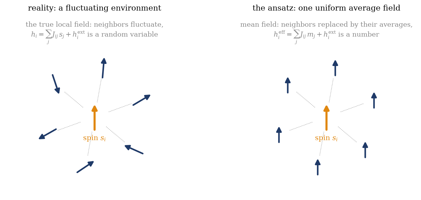
Figure 9.1 draws the physical idea. A spin in an interacting system feels the field of its neighbors — a fluctuating field, different in every configuration, correlated with the spin itself. Mean field replaces that fluctuating environment by its average: every neighbor \(s_j\) is frozen to its mean \(m_j\), and the spin responds to a single, deterministic effective field \(h_i^\text{eff} = \sum_j J_{ij} m_j + h_i\). The substitution would be exact if the neighbors did not fluctuate; its error is the fluctuation. Everything the approximation gets wrong — and the next lecture will show it getting a phase transition’s location and character wrong — traces back to this one sentence.

Figure 9.1: The central picture of Module 2’s opening, a century old. Left: reality — a spin’s local field is built from neighbors that fluctuate, so the field is a random variable, correlated with the spin it acts on. Right: the mean-field ansatz — every neighbor is replaced by its average magnetization, and the spin sits in a single deterministic effective field \(h_i^{\text{eff}} = \sum_j J_{ij} m_j + h_i\). The substitution is exact if the neighbors do not fluctuate; the error is precisely the fluctuation — which is why mean field improves with connectivity (many neighbors average sharply) and fails where fluctuations dominate.

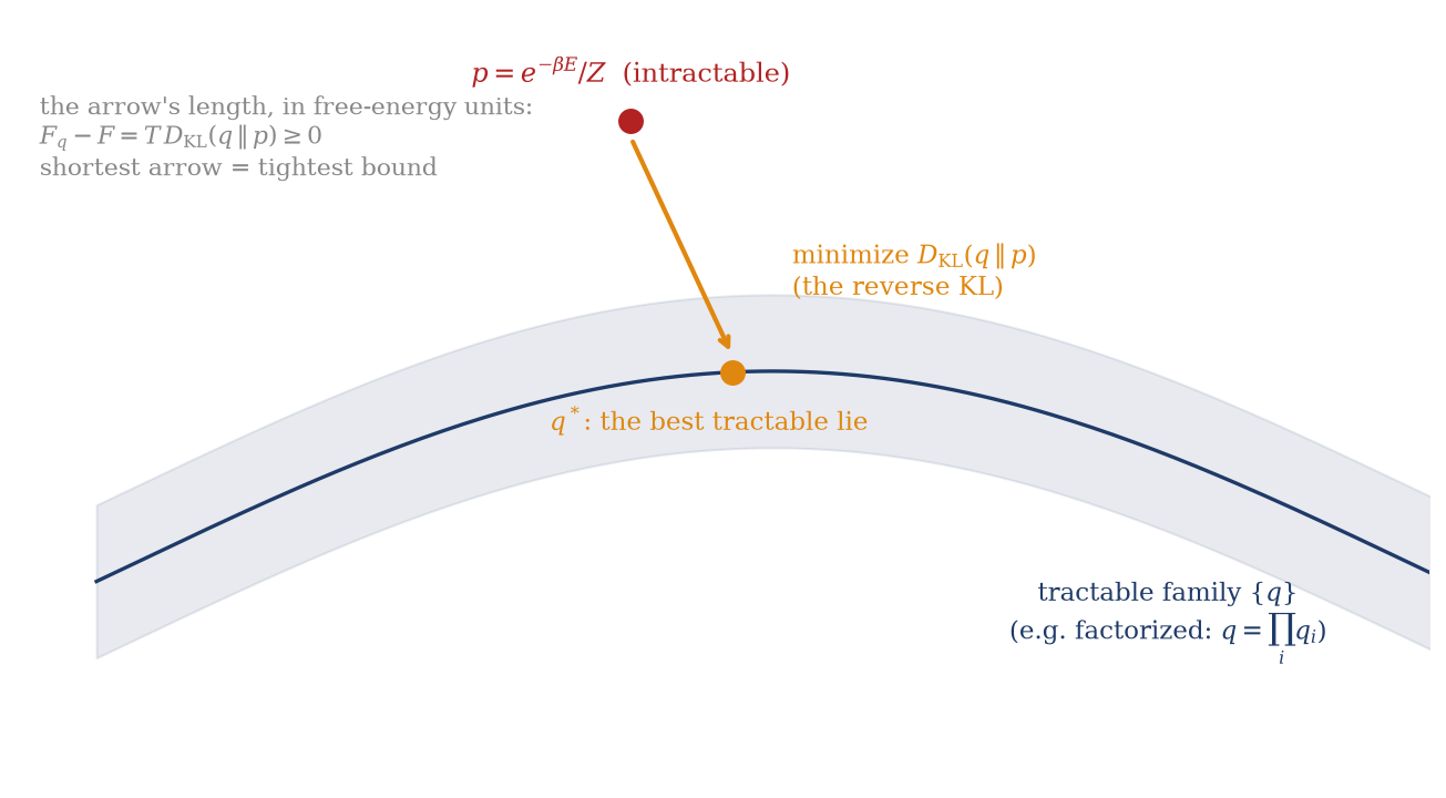
The formal version of the same move is a projection, and Figure 9.2 draws its geometry. The intractable \(p\) is a point in the space of distributions; the tractable candidates \(\{q\}\) — say, all factorized distributions — form a surface that does not contain it. Variational inference finds the point on the surface closest to \(p\), with distance measured by the Kullback–Leibler divergence — in a specific argument order whose consequences we will flag with a triangle. The next section supplies what the picture cannot: that the projection distance is exactly a free-energy difference, computable up to a constant without knowing \(Z\).

Figure 9.2: The variational principle as geometry: project the intractable \(p\) onto a tractable family. The projection minimizes the *reverse* KL divergence \(D_\mathrm{KL}(q\|p)\) — the only order we can average under — and the arrow’s length, measured in free-energy units, is the gap \(F_q - F = T\,D_\mathrm{KL}(q\|p) \geq 0\). Minimizing the variational free energy over the family therefore does two jobs at once: it finds the best tractable stand-in for \(p\), and it tightens a one-sided bound on the true free energy.

9.3 The engine, part I: the Gibbs–Bogoliubov bound

We want a functional of \(q\) that ① is computable whenever \(q\) is tractable, ② upper-bounds the intractable \(F\), and ③ touches it exactly at \(q = p\). Week 1 supplied every ingredient.

Define the variational free energy of an arbitrary trial distribution \(q(x)\) over the configurations:

\[ F_q \;\equiv\; \langle E \rangle_q \;-\; T\, S[q] \;=\; \sum_x q(x)\, E(x) \;+\; T \sum_x q(x) \log q(x). \]

This is Week 1’s free energy \(F = \langle E \rangle - TS\) with the Boltzmann distribution replaced by \(q\) in both terms — an energy cost plus an entropy price, evaluated under the wrong distribution. Note what is absent: no \(Z\). Every term is an average under \(q\), computable exactly for any tractable family.

Compute the gap to the true \(F = -T \log Z\). Insert \(\log Z\) under the \(q\)-average (it is a constant), and reassemble:

\[ F_q - F \;=\; \big\langle E + T \log q \big\rangle_q + T \log Z \;=\; T \Big\langle \log q + \beta E + \log Z \Big\rangle_q \;=\; T \Big\langle \log \frac{q(x)}{e^{-\beta E(x)}/Z} \Big\rangle_q \;=\; T \Big\langle \log \frac{q}{p} \Big\rangle_q . \]

Recognize the object on the right — it is the Kullback–Leibler divergence, and it is non-negative:

\[ \boxed{\; F_q - F \;=\; T\, D_\mathrm{KL}(q \,\|\, p) \;\geq\; 0, \qquad\text{so}\qquad F \;\leq\; F_q, \quad \text{with equality iff } q = p. \;} \tag{9.1}\]

Gibbs–Bogoliubov variational bound

The identity admits three readings. As a bound: the variational free energy never dips below the truth — equivalently \(\log Z \geq -F_q / T\), a lower bound on the log-partition function, the first quantitative grip the course has had on the normalizer. As an objective: minimizing \(F_q\) over a tractable family simultaneously tightens the bound on \(F\) and finds the member of the family closest to \(p\) in KL — one optimization serving both goals, which is why the method took hold in both fields. As a diagnostic: the gap is not vague “approximation error” but a named information-theoretic quantity, and when we can compute it (as in the example below) it tells us exactly how much distribution we have thrown away. (The classic physics statement of the same inequality — \(F \leq F_0 + \langle H - H_0 \rangle_0\) for a trial Hamiltonian \(H_0\), the Peierls–Bogoliubov form — is the special case \(q = e^{-\beta H_0}/Z_0\), traditionally proved from the convexity of the exponential, \(\langle e^X \rangle \geq e^{\langle X \rangle}\); the KL route above is the same mathematics with the inference reading built in, which is why we lead with it.)

Trap

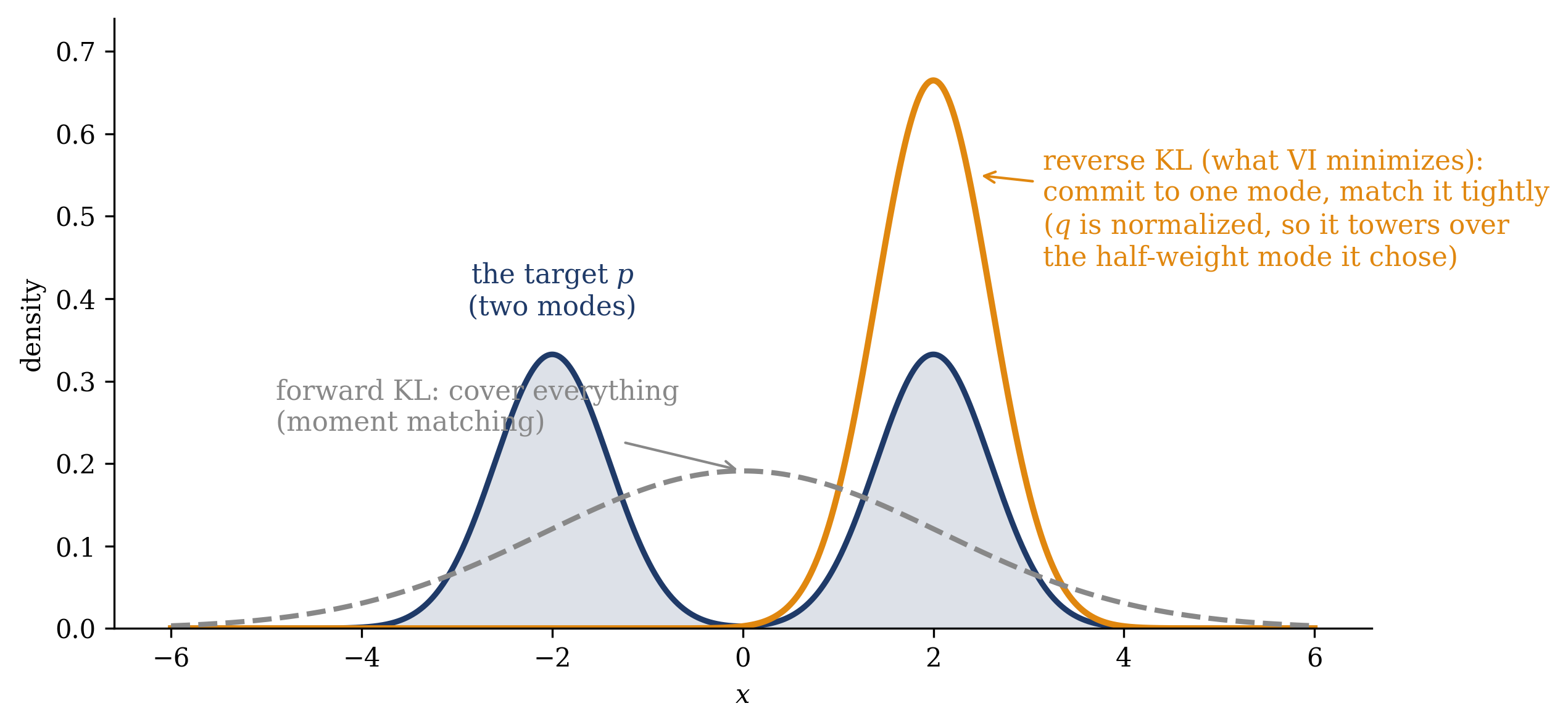
It is the reverse KL. The gap is \(D_\mathrm{KL}(q\|p)\) — averaged under \(q\) — not \(D_\mathrm{KL}(p\|q)\). The order is forced on us: we can only compute averages under the tractable distribution. But the two divergences penalize different sins. The reverse KL explodes where \(q\) puts mass and \(p\) has none, so the optimal \(q\) is mode-seeking: it commits to one region \(p\) likes and pays little for ignoring the others, and it systematically underestimates variance. The forward KL would instead spread \(q\) to cover everything (Figure 9.3). Every characteristic failure of the variational family of methods — mean field’s overconfident magnetizations below, the VAE’s posterior collapse in Week 7 — is this same asymmetry in another form. Know which divergence you are minimizing.

Show code

x = np.linspace(-6, 6, 2000)
dx = x[1] - x[0]
gauss = lambda x, mu, s: np.exp(-((x - mu) ** 2) / (2 * s**2)) / np.sqrt(2 * np.pi * s**2)
p = 0.5 * gauss(x, -2, 0.6) + 0.5 * gauss(x, 2, 0.6)

# forward KL optimum: moment matching (analytic)
mu_f, s_f = 0.0, np.sqrt(0.6**2 + 4.0)
# reverse KL optimum: grid search
best = (np.inf, 0, 1)
for mu in np.linspace(-3, 3, 121):
    for s in np.linspace(0.2, 3, 141):
        q = gauss(x, mu, s)
        kl = np.sum(q * np.log((q + 1e-300) / (p + 1e-300))) * dx
        if kl < best[0]:
            best = (kl, mu, s)
_, mu_r, s_r = best

fig, ax = plt.subplots(figsize=(8.6, 4.0))
ax.fill_between(x, p, color=NAVY, alpha=0.15)
ax.plot(x, p, color=NAVY, lw=2.2)
ax.plot(x, gauss(x, mu_r, s_r), color=ORANGE, lw=2.4)
ax.plot(x, gauss(x, mu_f, s_f), color=GRAY, ls="--", lw=2.0)
ax.text(-2.0, 0.38, r"the target $p$" "\n(two modes)", color=NAVY, fontsize=10.5, ha="center")
ax.annotate("reverse KL (what VI minimizes):\ncommit to one mode, match it tightly\n"
            "($q$ is normalized, so it towers over\nthe half-weight mode it chose)",
            xy=(2.45, 0.55), xytext=(3.15, 0.44), color=ORANGE, fontsize=10.5,
            arrowprops=dict(arrowstyle="->", color=ORANGE, lw=1))
ax.annotate("forward KL: cover everything\n(moment matching)",
            xy=(0.0, float(gauss(np.array([0.0]), mu_f, s_f)[0])),
            xytext=(-4.9, 0.24), color=GRAY, fontsize=10.5,
            arrowprops=dict(arrowstyle="->", color=GRAY, lw=1))
ax.set_xlabel(r"$x$"); ax.set_ylabel("density")
ax.set_ylim(0, 0.74)
fig.tight_layout(); plt.show()

Figure 9.3: The asymmetry of the two KL divergences, on the simplest instructive case: fit a single Gaussian \(q\) to a bimodal \(p\) (equal-weight modes at \(\pm 2\), width \(0.6\)). Minimizing the *forward* KL \(D_\mathrm{KL}(p\|q)\) (gray dashed) matches moments: the optimum straddles both modes, centered at zero with \(\sigma \approx 2.1\) — mass-covering, and placing most of its probability where \(p\) has almost none. Minimizing the *reverse* KL \(D_\mathrm{KL}(q\|p)\) (orange) — the divergence variational inference is forced to use — commits to a single mode and matches it tightly: mode-seeking, and blind to the mode it abandoned. Mean field’s overconfidence, and Week 7’s posterior collapse, are this picture at scale.

9.4 The engine, part II: the bound is the ELBO

The identification requires no new mathematics — only a redefinition of the energy.

Consider the machine-learner’s standard predicament: a latent-variable model \(p(x, z)\) — observed data \(x\), hidden variables \(z\) (cluster labels, latent codes, an RBM’s hidden layer) — whose fit to data is measured by the evidence \(p(x) = \sum_z p(x, z)\), and whose inferential heart is the posterior \(p(z \mid x) = p(x, z)/p(x)\). Both are intractable for the same reason \(Z\) was: the sum over \(z\).

Fix the observation \(x\) and manufacture an energy over the hidden variables — not a physical Hamiltonian, just a definition:

\[ E(z) \;\equiv\; -\log p(x, z), \qquad T = 1 . \]

Then the Boltzmann distribution of this energy is \(e^{-E(z)}/Z = p(x,z)/\sum_{z'} p(x,z')\) — the posterior — and its partition function is

\[ Z \;=\; \sum_z e^{-E(z)} \;=\; \sum_z p(x, z) \;=\; p(x) \]

— the evidence is a partition function. Every object in the variational construction now translates mechanically. The variational free energy of a trial \(q(z)\) becomes

\[ F_q \;=\; \langle E \rangle_q + \langle \log q \rangle_q \;=\; -\Big[ \big\langle \log p(x, z) \big\rangle_q - \big\langle \log q(z) \big\rangle_q \Big] \;=\; -\,\mathrm{ELBO}(q), \]

minus the machine-learner’s evidence lower bound, term for term. And the master identity Equation 9.1, transcribed, is the ELBO inequality with its exact gap:

\[ F_q = -\,\mathrm{ELBO}(q), \qquad F = -\log p(x), \qquad \log p(x) - \mathrm{ELBO}(q) = D_\mathrm{KL}\big(q(z)\,\big\|\, p(z \mid x)\big). \tag{9.2}\]

variational free energy ≡ negative ELBO

So \(F \leq F_q\) is \(\log p(x) \geq \mathrm{ELBO}\): maximizing the evidence lower bound is minimizing a variational free energy — the same functional under a substitution of symbols, not merely an analogy. The physicist bounding \(\log Z\) from below and the machine-learner bounding the log-evidence from below are running one optimization; Weiss’s molecular field and the inference engine inside every VAE are one method met at two ends of a century. Here is the dictionary in full — the dictionary for the next three weeks:

Table 9.1: The physics ⇄ inference dictionary: one functional, two vocabularies.

statistical physics	variational inference
configuration \(x\)	latent variable \(z\) (data \(x\) fixed)
energy \(E(x)\)	\(-\log p(x, z)\)
Boltzmann distribution \(p = e^{-\beta E}/Z\)	posterior \(p(z \mid x)\)
partition function \(Z\)	evidence \(p(x)\)
free energy \(F = -T\log Z\)	negative log-evidence \(-\log p(x)\)
trial distribution \(q(x)\)	variational posterior \(q(z)\)
variational free energy \(F_q\)	\(-\,\mathrm{ELBO}(q)\)
gap \(T\, D_\mathrm{KL}(q\\|p)\)	\(\log p(x) - \mathrm{ELBO}\)
minimize the free energy	variational inference

9.5 The engine, part III: mean field, the factorized ansatz

The bound holds for any \(q\); it becomes a method the moment we commit to a family. Take the simplest tractable one: complete independence,

\[ q(s) \;=\; \prod_{i=1}^{N} q_i(s_i), \qquad q_i(s_i) = \frac{1 + m_i s_i}{2}, \]

for Ising variables \(s_i = \pm 1\), parameterized by the per-spin magnetizations \(m_i = \langle s_i \rangle_q \in [-1, 1]\) — these are the variational parameters we will optimize. (A hygiene note: this \(m_i\) is a variational per-site magnetization, a knob we turn; Week 2’s overlap \(m\) was an order parameter of the true dynamics. Same letter, same physical flavor, different formal role.)

Evaluate the two halves of \(F_q\) for the Ising energy \(E = -\tfrac12 \sum_{i \neq j} J_{ij} s_i s_j - \sum_i h_i s_i\). The energy term is where the approximation acts: under a factorized \(q\), expectations of products split,

\[ \langle s_i s_j \rangle_q = m_i m_j \quad (i \neq j) \qquad\Longrightarrow\qquad \langle E \rangle_q \;=\; -\tfrac{1}{2} \sum_{i \neq j} J_{ij}\, m_i m_j \;-\; \sum_i h_i m_i . \]

Read the first equality as the approximation stated as an equation: the factorization sets every connected correlation \(\langle s_i s_j \rangle - \langle s_i \rangle \langle s_j \rangle\) to zero — identically, not merely approximately. That is the entire price of tractability, localized in one line. The entropy term, by contrast, is exact for the family and splits by independence into a sum of binary entropies,

\[ S[q] \;=\; \sum_i s(m_i), \qquad s(m) = -\frac{1+m}{2} \log\frac{1+m}{2} - \frac{1-m}{2} \log\frac{1-m}{2}. \]

Now minimize \(F_q = \langle E \rangle_q - T \sum_i s(m_i)\) over each \(m_i\). The energy contributes \(\partial \langle E \rangle_q / \partial m_i = -\big( \sum_j J_{ij} m_j + h_i \big) \equiv -h_i^\text{eff}\) (the \(\tfrac12\) canceling the \(ij\)/\(ji\) double count, the same bookkeeping as Week 3’s gradient); the entropy contributes \(\partial s(m_i)/\partial m_i = -\operatorname{artanh}(m_i)\) (differentiate the binary entropy and the logs collapse). Stationarity, \(-h_i^\text{eff} + T \operatorname{artanh}(m_i) = 0\), then inverts to

\[ \boxed{\; m_i \;=\; \tanh\!\Big( \beta \Big( \sum_j J_{ij}\, m_j + h_i \Big) \Big) \;} \tag{9.3}\]

mean-field self-consistent equations

— the mean-field equations, and the cartoon of Figure 9.1 now derived rather than drawn. Each spin responds — with Week 1’s exact two-state Boltzmann average, the \(\tanh\) — to the average field of its neighbors rather than their fluctuating states. And the equations are self-consistent: the magnetizations determine the effective fields that determine the magnetizations, a loop closed on itself. That loop is where all the physics of the next lecture lives — a closed loop can sustain a solution with no external cause, which is what spontaneous magnetization is.

The equation admits two readings. Physics reading: this is Weiss’s molecular-field equation of 1907 (Weiss 1907) — but where Weiss posited the average field, we have derived it as the optimum of a variational bound, so we know exactly what was discarded (the correlations) and in which direction the answer errs (\(F_q \geq F\), always). Inference reading: iterate the equations — sweep the sites, update each \(m_i \leftarrow \tanh(\beta h_i^\text{eff})\) from the current neighbors — and you are running naive mean-field variational inference, coordinate ascent on the ELBO, each update provably lowering \(F_q\) (the monotonicity is one line from the bound: each \(m_i\)-update is an exact minimization of \(F_q\) in that coordinate with the others frozen; the general-family version of the update, \(q_i \propto \exp \langle \log p \rangle_{q_{\setminus i}}\), is the CAVI algorithm of the ML textbooks (Blei, Kucukelbir, and McAuliffe 2017)). The 1907 self-consistency and the 2017 inference algorithm are the same fixed-point iteration.

When should the lie be a good one? The cartoon answers: mean field is the exact theory of a system whose spins do not fluctuate about their means, so its quality is set by the sharpness of the average field. A spin with \(z\) neighbors feels an effective field that is a sum of \(z\) terms; its relative fluctuation scales as \(1/\sqrt{z}\). High connectivity — high dimension, dense graphs, the fully-connected models of Weeks 2–4, and (not coincidentally) the wide dense layers of modern machine learning — is mean field’s home turf. Low dimension and the vicinity of a critical point, where fluctuations are the whole story, are where it fails — instructively, as the next lecture will show. And one more standing warning: the self-consistent equations may have several solutions (that multiplicity is exactly how the phase transition will appear); the variational principle adjudicates — take the solution with the lowest \(F_q\).

Take-home 2

The factorized ansatz \(q = \prod_i q_i\) turns the bound into mean-field theory: \(F_q\) is minimized at \(m_i = \tanh\big(\beta(\sum_j J_{ij} m_j + h_i)\big)\) — each spin in the average field of its neighbors. The price is exact and structural: all connected correlations are set to zero. Iterating the equations is naive mean-field variational inference, monotonically descending \(F_q\); the approximation is best at high connectivity (\(1/\sqrt{z}\) field fluctuations) and worst near criticality.

9.6 Example: the bound in action

One small model where the truth is computable, so that for once the bound, the gap, and the discarded correlations are all visible. Take \(N = 6\) spins, fully connected with ferromagnetic couplings \(J_{ij} = J_0/N\) (\(J_0 = 1\) — the model the next lecture pushes to its \(N \to \infty\) limit), plus a small symmetry-breaking field \(h = 0.05\). With \(2^6 = 64\) states, exact enumeration gives \(Z\), \(F\), and every moment; solving Equation 9.3 by iteration gives the mean-field \(m_i\) and \(F_q\). The comparison, across temperature:

\(T\)	exact \(F\)	mean-field \(F_q\)	gap \(= T\,D_\mathrm{KL}(q\\|p)\)	exact \(\langle s_i \rangle\)	mean-field \(m_i\)
\(3.0\)	\(-12.561\)	\(-12.480\)	\(0.081\)	\(0.023\)	\(0.023\)
\(1.0\)	\(-4.514\)	\(-4.201\)	\(0.313\)	\(0.131\)	\(0.262\)
\(0.7\)	\(-3.519\)	\(-3.214\)	\(0.305\)	\(0.263\)	\(0.742\)
\(0.3\)	\(-2.844\)	\(-2.805\)	\(0.039\)	\(0.754\)	\(0.994\)

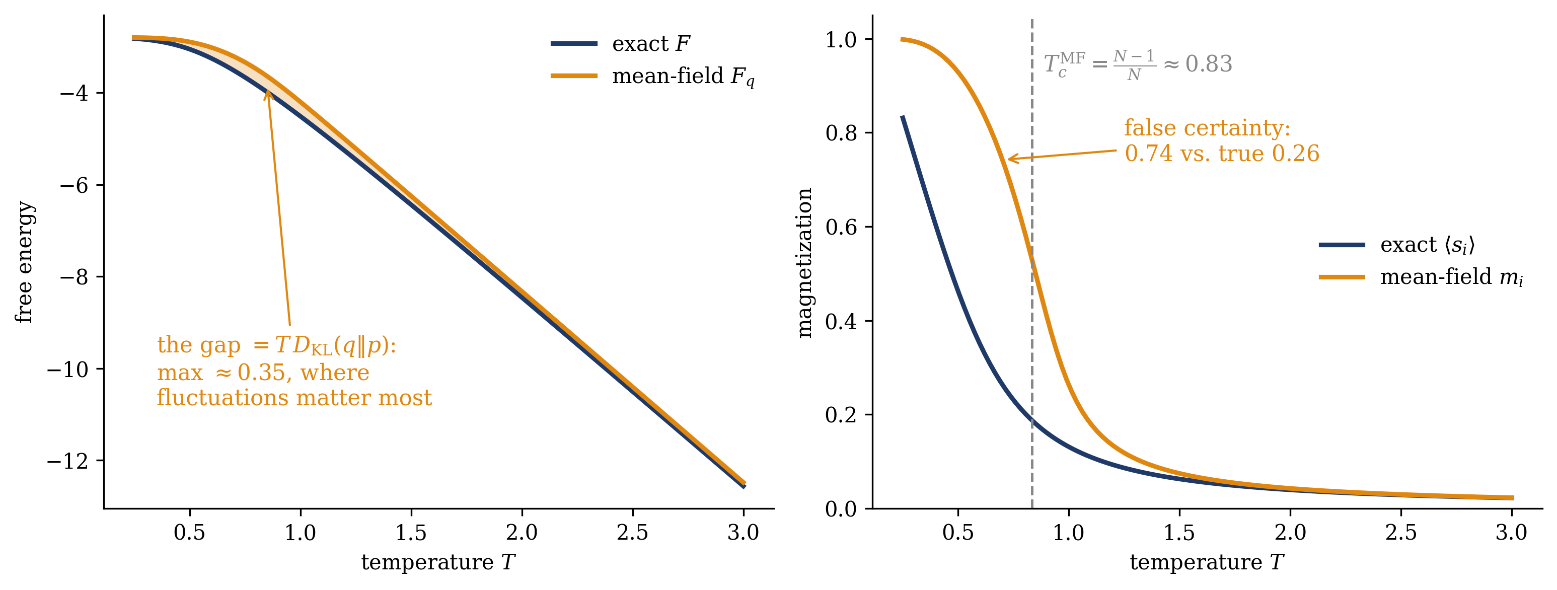
Read the table by columns, because each column checks one claim of the lecture. The gap column is never negative — the bound Equation 9.1, made numerical (and computed two independent ways in the code below: as \(F_q - F\), and directly as \(T \sum_s q \log(q/p)\) over all \(64\) states; they agree to machine precision, which is the identity Equation 9.1 verified rather than trusted). The gap is small at high temperature, where spins are nearly independent and the factorized family nearly contains the truth; small again at very low temperature, where the system freezes into an essentially factorized ordered state; and largest in between — peaking at \(0.35\) near \(T \approx 0.85\), a tenth of the free energy — precisely where correlated fluctuations are strongest. The magnetization columns show the reverse-KL signature we promised: at \(T = 0.7\) the exact magnetization is a modest \(0.26\), but mean field reports \(0.74\) — the factorized \(q\), unable to spend probability on correlated fluctuations, buys its free energy by overcommitting to order, the mode-seeking overconfidence of Figure 9.3 realized in spins. Figure 9.4 draws both columns as curves, and marks the temperature \(T_c^\text{MF} = (N-1)J_0/N \approx 0.83\) where the next lecture will have much to say: mean field manufactures a sharp onset of order there, while the exact six-spin system — which, being finite, has no phase transition at all — crosses over smoothly. The gap peaks in exactly that neighborhood. Where the approximation manufactures a sharp transition is where it is least trustworthy — a diagnosis the next lecture turns into theory, and the tutorial into a projector experiment.

Show code

N, J0, h = 6, 1.0, 0.05
J = J0 / N * (np.ones((N, N)) - np.eye(N))
S = np.array([[(c >> i & 1) * 2 - 1 for i in range(N)] for c in range(2**N)], dtype=float)
E = -0.5 * np.einsum("ci,ij,cj->c", S, J, S) - h * S.sum(axis=1)

def exact(T):
    w = np.exp(-E / T)
    Z = w.sum(); p = w / Z
    return -T * np.log(Z), (p[:, None] * S).sum(axis=0)[0], p

def meanfield(T):
    m = np.full(N, 0.9)
    for _ in range(5000):
        m_new = np.tanh((J @ m + h) / T)
        if np.abs(m_new - m).max() < 1e-12:
            break
        m = 0.7 * m + 0.3 * m_new
    Eq = -0.5 * m @ J @ m - h * m.sum()
    Sq = np.sum(-(1 + m) / 2 * np.log((1 + m) / 2) - (1 - m) / 2 * np.log((1 - m) / 2))
    return Eq - T * Sq, m

Ts = np.linspace(0.25, 3.0, 120)
Fex, Fq, mex, mmf = [], [], [], []
for T in Ts:
    F, m0, p = exact(T)
    Fqv, m = meanfield(T)
    q = np.prod((1 + S * m) / 2, axis=1)          # the factorized q, enumerated
    assert abs((Fqv - F) - T * (q * np.log(q / p)).sum()) < 1e-8   # gap = T*KL, verified
    Fex.append(F); Fq.append(Fqv); mex.append(m0); mmf.append(m[0])
Fex, Fq, mex, mmf = map(np.array, (Fex, Fq, mex, mmf))
Tc = (N - 1) * J0 / N

fig, (a1, a2) = plt.subplots(1, 2, figsize=(10.4, 4.0))
a1.plot(Ts, Fex, color=NAVY, lw=2.2, label=r"exact $F$")
a1.plot(Ts, Fq, color=ORANGE, lw=2.2, label=r"mean-field $F_q$")
a1.fill_between(Ts, Fex, Fq, color=ORANGE, alpha=0.25)
k = np.argmax(Fq - Fex)
a1.annotate(rf"the gap $= T\,D_{{\rm KL}}(q\|p)$:"
            f"\nmax $\\approx {np.max(Fq-Fex):.2f}$, where"
            "\nfluctuations matter most",
            xy=(Ts[k], (Fex[k] + Fq[k]) / 2), xytext=(0.35, -10.8),
            color=ORANGE, fontsize=10.5,
            arrowprops=dict(arrowstyle="->", color=ORANGE, lw=1))
a1.set_xlabel(r"temperature $T$"); a1.set_ylabel("free energy")
a1.legend(frameon=False, fontsize=10, loc="upper right")
a2.plot(Ts, mex, color=NAVY, lw=2.2, label=r"exact $\langle s_i\rangle$")
a2.plot(Ts, mmf, color=ORANGE, lw=2.2, label=r"mean-field $m_i$")
a2.axvline(Tc, color=GRAY, ls="--", lw=1.2)
a2.text(Tc + 0.05, 0.93, r"$T_c^{\rm MF} = \frac{N-1}{N} \approx 0.83$",
        color=GRAY, fontsize=10.5)
a2.annotate("false certainty:\n$0.74$ vs. true $0.26$", xy=(0.7, 0.742),
            xytext=(1.25, 0.74), color=ORANGE, fontsize=10.5,
            arrowprops=dict(arrowstyle="->", color=ORANGE, lw=1))
a2.set_xlabel(r"temperature $T$"); a2.set_ylabel("magnetization")
a2.set_ylim(0, 1.05)
a2.legend(frameon=False, fontsize=10, loc="center right")
fig.tight_layout(); plt.show()

Figure 9.4: The bound in action: exact versus mean-field thermodynamics of a fully-connected \(N = 6\) ferromagnet (\(J_{ij} = 1/N\), \(h = 0.05\)), exact values from enumeration of all \(64\) states. Left: the true free energy \(F\) (navy) and the variational \(F_q\) (orange) — \(F_q\) never dips below \(F\), and the shaded gap, equal to \(T\,D_\mathrm{KL}(q\|p)\) by Equation 9.1 (verified in the code by direct enumeration of the KL), peaks at \(\approx 0.35\) near the mean-field critical temperature and closes at both ends. Right: the magnetizations. Mean field (orange) switches on sharply near \(T_c^{\mathrm{MF}} = (N{-}1)/N \approx 0.83\) (dashed) — a phase transition it has manufactured — while the exact finite system (navy) crosses over smoothly; at \(T = 0.7\) the approximation reports \(m = 0.74\) against a true \(0.26\). Overconfident order is the reverse-KL signature: the factorized family cannot afford fluctuations, so it buys free energy with false certainty.

The mean-field free energy is never below the truth — that is the guarantee: we are always wrong in one known direction, by exactly a KL divergence.

The next lecture takes Equation 9.3 to the ferromagnet proper — uniform couplings, \(h = 0\), \(N \to \infty\) — where a nonzero magnetization appears spontaneously below a critical temperature: a phase transition, falling out of a variational approximation, with an order parameter and a critical exponent. The tutorial then puts mean field, Monte Carlo sampling, and exact enumeration side by side on one small lattice, testing where the three agree and where the bound opens a gap.

Take-home 3

On a brute-forceable model the guarantee is visible: \(F_q \geq F\) at every temperature, by exactly \(T\,D_\mathrm{KL}(q\|p)\), with the gap largest where correlated fluctuations are strongest — near the transition mean field itself manufactures — and the mean-field magnetizations overconfident there (reverse-KL mode-seeking, in spins). Exact at weak coupling; wrong, in one known direction, elsewhere.

9.7 Outlook: a phase transition from an approximation

Confronted with an intractable \(Z\), we traded the true distribution for a tractable approximation — chosen by minimizing a one-sided bound whose gap is a KL divergence — and found that the physicist’s version of this trade (Gibbs–Bogoliubov, Weiss’s molecular field) and the machine-learner’s (the ELBO, variational inference) are one functional under two names. The dictionary of Table 9.1 applies throughout Module 2.

The next lecture applies the method to the uniform ferromagnet: the self-consistency \(m = \tanh(\beta z J m)\) breaks symmetry — below \(T_c = zJ\) the disordered solution destabilizes and the system magnetizes spontaneously, with the square-root onset \(m \sim (T_c - T)^{1/2}\) — a genuine collective phase transition, predicted by an approximation that ignores every correlation. But the same approximation overestimates \(T_c\) (it ignores the fluctuations that fight order), predicts a transition even in one dimension where none exists, and gets the critical exponents wrong — because at criticality fluctuations are not a correction but the dominant effect. Restoring the discarded correlations systematically is Week 6’s agenda: the TAP correction (Thouless, Anderson & Palmer 1977, who corrected the very Sherrington–Kirkpatrick model Week 2 leaned on) and belief propagation, which is exact on trees. The machine-learning arrow runs parallel: naive mean-field VI is the workhorse of scalable Bayesian inference, and its mode-seeking bias becomes Week 7’s posterior collapse inside the variational autoencoder.