5 The Boltzmann machine: learning meets the partition function

5.1 Week 2’s promise, redeemed

Week 2 ended on a promissory note: replace the deterministic update Equation 3.1 by a coin flip — flip spin \(k\) with probability \(1/(1 + e^{\beta \Delta E})\) — and two things follow. First, the stationary distribution of this dynamics is exactly Week 1’s Boltzmann law over the network’s energy: the two halves of the course so far click together. Second, the moment we ask the network to learn its couplings from data by maximum likelihood — rather than have Hebb write them by fiat — the gradient acquires a term that requires \(Z\). Both are proved below.

The history hook is the other half of the 2024 Nobel: Week 2 opened on the Hopfield half; today is the Hinton half. Ackley, Hinton, and Sejnowski (1985) took Hopfield’s Ising network, made it stochastic, gave it a learning algorithm, and named the result after the distribution at its heart: the Boltzmann machine. The lineage traced in Chapter 1 thus closes its longest loop — Boltzmann’s counting in the 1870s, Gibbs’s partition function in 1902, Hopfield’s landscape in 1982, and now, 1985, a machine that carries Boltzmann’s name and learns a probability distribution from examples. The citation honors this as physics: the machine is an Ising model, its dynamics is Glauber’s, and its failure mode is a partition function.

The question is one step past Week 2’s. That network remembered what we wrote into it — Hebb’s rule Equation 3.4 is a storage prescription, not a learning algorithm. Can a network learn what to remember — discover its own couplings from data alone? Yes, by a short rule — a few lines of calculus. The price is the obstruction the course is organized around: \(Z\), named in Chapter 1 as the training obstruction of Module 1, is here derived and pinned to a precise mathematical object.

Module 1’s arc is measure \(E\) (Week 1) → design \(E\) (Week 2) → learn \(E\) (Week 3), and this lecture completes it. A deeper symmetry runs through the argument: Week 1 derived the Boltzmann distribution from maximum entropy with the energy given (Section 1.4); here we run that derivation backwards — the data supply the constraints, and out fall both the learning rule and its obstruction. The course’s opening derivation and its first learning algorithm turn out to be one theorem seen from two sides.

Take-home 1

A Boltzmann machine is Week 2’s network heated up (Glauber dynamics \(\Rightarrow\) Boltzmann stationary law) and made trainable (couplings fit to data by maximum likelihood). Memorizing — Hebb, one shot, no objective — becomes learning: gradient ascent on the likelihood. The step from design to learn is the step that brings in \(Z\).

5.2 Memorize versus learn

Two dichotomies organize what follows.

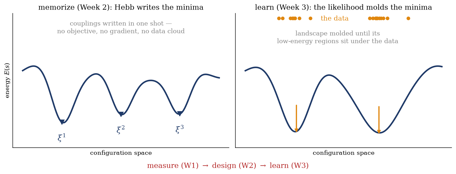
The first is memorize versus learn, drawn in Figure 5.1. Hebb’s rule Equation 3.4 writes the couplings in a single pass over the patterns: no objective function to descend and no iteration — the minima of the landscape are placed, once, at prescribed locations. Maximum likelihood inverts the logic. We posit a model distribution \(p(s) = e^{-\beta E(s)}/Z\) whose energy carries free parameters \((J, \theta)\), and we choose those parameters to maximize the probability the model assigns to the training data. The couplings are no longer written; they are fit, and the landscape is molded — iteratively, under an objective — until its low-energy regions sit under the data. Hebb, in this light, is a special, cheap, often-suboptimal solution to a problem maximum likelihood poses properly; we will meet Hebb again inside the exact learning rule, as one of its two terms.

Figure 5.1: The module’s last turn: from couplings written to couplings fit. Left: Hebb (Week 2) places the minima at prescribed patterns \(\xi^\mu\) in one shot — no objective and no iteration. Right: maximum likelihood (this week) posits an energy with free parameters and molds the landscape under an objective until its basins sit beneath the data. The objective is the log-likelihood, and its gradient is the subject of this lecture — the two forces of Figure 5.2.

The second dichotomy is the one the rest of the course keeps returning to: positive phase versus negative phase. Every gradient we write today is a difference of two brackets — an average over the data (“what the world shows you”) and an average over the model (“what the network dreams up”). Hinton’s informal names, the wake phase and the sleep phase, are a serviceable mnemonic (not to be confused with the later wake–sleep algorithm for Helmholtz machines, Dayan et al. (1995), a different construction); positive and negative phase, the terms of Ackley, Hinton, and Sejnowski (1985), are the technical vocabulary we keep. One of the two brackets is trivial to compute; the other is the wall — and telling them apart is the argument below.

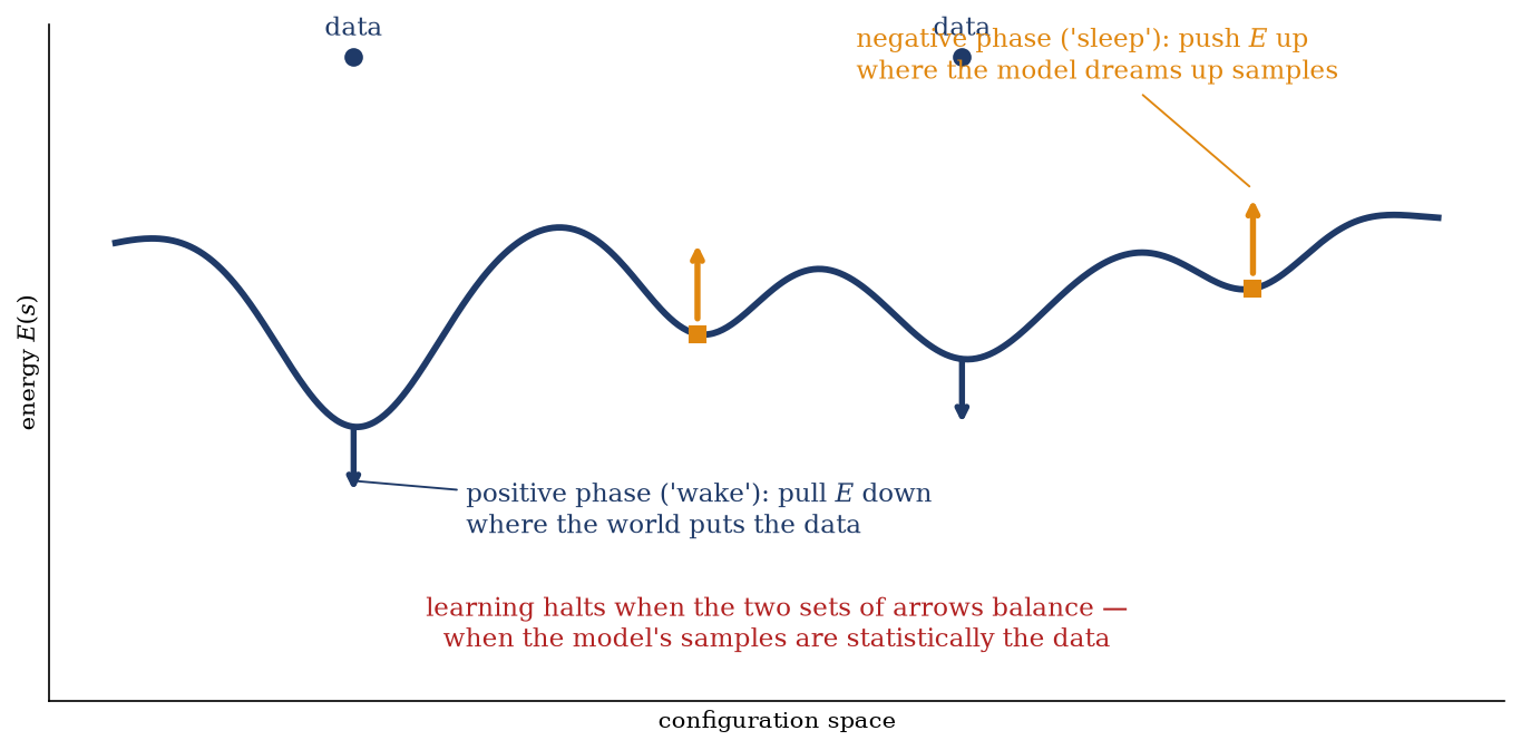
Figure 5.2 draws the central picture; every result below is a refinement of it — a single energy landscape over configuration space. At each data point, an arrow pulling the energy down: make what you saw more probable. At each model sample — each fantasy the network dreams on its own — an arrow pushing the energy up: make what you merely imagined less probable. Learning halts when the two sets of arrows balance, which happens precisely when the model’s fantasies are statistically indistinguishable from the data. Training is down on data, up on dreams.

Figure 5.2: The central picture of the lecture, drawn before the mathematics. Training a Boltzmann machine exerts two forces on the energy landscape: the positive (“wake”) phase pulls \(E\) down at the data, making the observed configurations more probable; the negative (“sleep”) phase pushes \(E\) up at the model’s own samples, making its fantasies less probable. The gradient we derive below is exactly this pair of forces, and learning stops when they balance — when sampling the model is statistically like sampling the data. The negative arrows are the expensive ones: finding where the model dreams requires \(Z\).

Three results make this precise: ① the model distribution, and why it is Boltzmann (Section 5.3); ② the exact form of the two forces — the maximum-likelihood gradient (Section 5.4); ③ why the “up on dreams” force is the expensive one (Section 5.5).

5.3 Heating the network up: Glauber dynamics

The dynamics comes first. Week 2’s network ran at zero temperature — the update Equation 3.1 was the locally greedy choice, and the Lyapunov theorem of Section 3.4 rewarded it with deterministic descent. Now heat it up, following Glauber (1963). The energy is Week 2’s, with one addition: the thresholds we set to zero there return as learnable biases (physics dialect: local fields),

\[ E(s) \;=\; -\tfrac{1}{2} \sum_{i \neq j} J_{ij}\, s_i s_j \;-\; \sum_i \theta_i\, s_i, \qquad J_{ij} = J_{ji}, \quad J_{ii} = 0. \tag{5.1}\]

Boltzmann-machine energy

A notation flag before we move: \(\theta_i\) is a bias — one learnable parameter of the energy — and when we later write \(\nabla_\theta\) for “the gradient with respect to all parameters,” it ranges over the full collection \((J, \theta)\). As Chapter 1 warned, symbols will be overloaded; this is the first collision that matters.

The stochastic update. Pick a site \(k\) at random — asynchronously, as in Week 2 — and propose the flip \(s_k \to -s_k\). The flip costs \(\Delta E_k = 2\, s_k h_k\), where \(h_k = \sum_j J_{kj} s_j + \theta_k\) is the local field (the same \(\Delta E\) that ran the Lyapunov argument). Accept the flip with probability

\[ w(s_k \to -s_k) \;=\; \frac{1}{1 + e^{\beta \Delta E_k}} \tag{5.2}\]

Glauber flip rule

— downhill moves are accepted gladly (\(w \to 1\) for \(\Delta E \ll -T\)), uphill moves reluctantly but not never (\(w \to 0\) only as \(\Delta E/T \to \infty\)), and as \(\beta \to \infty\) the rule collapses onto Week 2’s greedy \(\operatorname{sign}(h_k)\). Equivalently, the rule sets

\[ p(s_k = +1 \mid s_{\setminus k}) \;=\; \frac{1}{1 + e^{-2\beta h_k}} \;=\; \sigma(2\beta h_k) \]

— the logistic function, which you last met as the two-state Boltzmann occupation in Section 1.6. The “activation function” of every neural network is, here, literally a conditional Boltzmann probability for a two-state degree of freedom in the field of its neighbors.

Detailed balance, in three lines. Where does this dynamics settle? Consider two configurations \(s\) and \(s'\) that differ at the single site \(k\), and take the ratio of forward and backward flip probabilities. With \(\Delta E = E(s') - E(s)\), the reverse move costs \(-\Delta E\), so

\[ \frac{w(s \to s')}{w(s' \to s)} \;=\; \frac{1 + e^{-\beta \Delta E}}{1 + e^{\beta \Delta E}} \;=\; e^{-\beta \Delta E} \,\frac{e^{\beta \Delta E} + 1}{1 + e^{\beta \Delta E}} \;=\; e^{-\beta\left[ E(s') - E(s) \right]}. \]

The transition probabilities therefore satisfy detailed balance, \(p(s)\, w(s \to s') = p(s')\, w(s' \to s)\), with respect to exactly one distribution:

\[ p(s) \;=\; \frac{e^{-\beta E(s)}}{Z}, \qquad Z = \sum_s e^{-\beta E(s)} \tag{5.3}\]

the model distribution

— and a distribution satisfying detailed balance is stationary: the probability flowing out of any state along each single-flip edge is exactly balanced by the flow back in. In words: Week 1’s Boltzmann distribution has returned — but where Week 1 handed us the energy, here \(E\) carries free parameters we are about to fit, and \(Z\) is the normalizer we will spend the rest of the course working around. Heating the network up is what turns a memory into a probability distribution over configurations: the machine no longer sits in one minimum; it visits configurations with Boltzmann weights, and can be asked what it thinks is likely.

Two caveats, one sentence each. Stationarity plus irreducibility (any state reachable from any state — true here, since every \(w > 0\) at finite \(T\)) and aperiodicity guarantee that the chain converges to Equation 5.3 from any start; asynchronous random-site updating supplies both, and we take the ergodic bookkeeping as read. How fast it converges — the mixing time — is an entirely separate matter, and we flag now that it returns as the second obstruction in Section 5.5. Finally, the temperature: \(\beta\) multiplies parameters we are about to learn, so it can be absorbed into them — a machine at \(\beta = 2\) with couplings \(J\) is the same model as a machine at \(\beta = 1\) with couplings \(2J\). We set \(\beta = 1\) from here on and say so once.

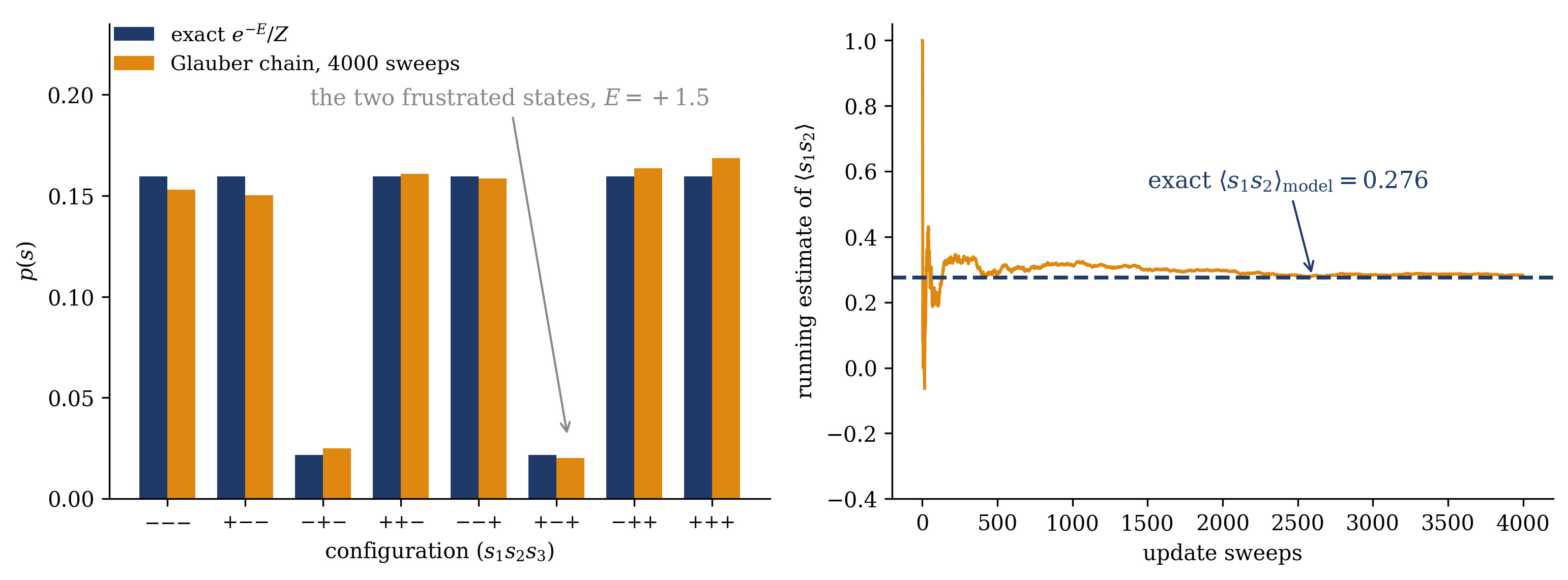
Figure 5.3 shows the theorem at work on a machine small enough to check exhaustively — three spins, the same frustrated triangle we dissect by hand in Section 5.7: the empirical visit frequencies of the Glauber chain converge onto the eight exact Boltzmann probabilities, and a running average over the chain converges onto the exact model expectation \(\langle s_1 s_2 \rangle_\text{model}\). The fluctuating line in the right panel — an expectation estimated by running the dynamics — is precisely the object the learning rule of Section 5.4 demands, once per gradient step.

Show code

rng = np.random.default_rng(7)
J = np.array([[0.0, 0.5, -0.5], [0.5, 0.0, 0.5], [-0.5, 0.5, 0.0]])

# exact enumeration: 8 configurations, energies, Boltzmann weights
S = np.array([[(c >> i & 1) * 2 - 1 for i in range(3)] for c in range(8)])
E = -0.5 * np.einsum("ci,ij,cj->c", S, J, S)
p_exact = np.exp(-E) / np.exp(-E).sum()
s1s2_exact = (S[:, 0] * S[:, 1] * p_exact).sum()          # = 0.2758

# one Glauber chain: random site, flip with prob 1/(1+e^{dE})
n_updates = 3 * 4000                                       # 4000 sweeps
s = np.ones(3)
visits = np.zeros(8)
running = np.empty(n_updates)
acc = 0.0
for t in range(n_updates):
    k = rng.integers(3)
    dE = 2 * s[k] * (J[k] @ s)
    if rng.random() < 1 / (1 + np.exp(dE)):
        s[k] = -s[k]
    visits[int((s[0] > 0) + 2 * (s[1] > 0) + 4 * (s[2] > 0))] += 1
    acc += s[0] * s[1]
    running[t] = acc / (t + 1)

fig, (a1, a2) = plt.subplots(1, 2, figsize=(10.4, 3.9))
labels = ["".join("+" if x > 0 else "$-$" for x in c) for c in S]
xpos = np.arange(8)
a1.bar(xpos - 0.18, p_exact, width=0.36, color=NAVY, label=r"exact $e^{-E}/Z$")
a1.bar(xpos + 0.18, visits / n_updates, width=0.36, color=ORANGE,
       label="Glauber chain, 4000 sweeps")
a1.set_xticks(xpos, labels, fontsize=9)
a1.set_xlabel(r"configuration $(s_1 s_2 s_3)$"); a1.set_ylabel(r"$p(s)$")
a1.set_ylim(0, 0.235)
a1.annotate("the two frustrated states, $E = +1.5$", xy=(5.15, 0.03), xytext=(4.4, 0.195),
            color=GRAY, fontsize=10.5, ha="center",
            arrowprops=dict(arrowstyle="->", color=GRAY, lw=1))
a1.legend(frameon=False, fontsize=9.5, loc="upper left", bbox_to_anchor=(-0.02, 1.04))
a2.plot(np.arange(n_updates) / 3, running, color=ORANGE, lw=1.4)
a2.axhline(s1s2_exact, color=NAVY, ls="--", lw=1.8)
a2.annotate(rf"exact $\langle s_1 s_2\rangle_\mathrm{{model}} = {s1s2_exact:.3f}$",
            xy=(2600, s1s2_exact), xytext=(1500, 0.55), color=NAVY, fontsize=11,
            arrowprops=dict(arrowstyle="->", color=NAVY, lw=1))
a2.set_xlabel("update sweeps"); a2.set_ylabel(r"running estimate of $\langle s_1 s_2\rangle$")
a2.set_ylim(-0.4, 1.05)
fig.tight_layout(); plt.show()

Figure 5.3: Glauber dynamics finding the Boltzmann distribution, on the \(N = 3\) machine of Section 5.7 (\(J_{12} = J_{23} = 0.5\), \(J_{13} = -0.5\), \(\theta = 0\); \(Z = 10.34\)). Left: exact Boltzmann probabilities \(e^{-E(s)}/Z\) of the eight configurations (navy) against the visit frequencies of a single Glauber chain of \(4000\) sweeps (orange) — the six degenerate low-energy states at \(E = -0.5\) and the two frustrated states at \(E = +1.5\) are all reproduced. Right: the running chain estimate of \(\langle s_1 s_2 \rangle\) converging onto the exact model expectation \(0.276\) (dashed). This fluctuating estimate is exactly what the learning rule of Section 5.4 demands: a model expectation, re-estimated at every gradient step.

5.4 The engine: the maximum-likelihood gradient

To fit \((J, \theta)\) we need an objective and its gradient. The objective writes itself; but \(\log p\) contains \(-\log Z\), and \(Z\) depends on every parameter, so the gradient will contain \(\partial \log Z / \partial(J, \theta)\) — and that term will not go away. We meet it by computing it.

Setup. The data are \(D\) configurations \(\mathcal{D} = \{s^{(1)}, \dots, s^{(D)}\}\) — binarized images, spike patterns, spin snapshots — treated as independent draws. The (average) log-likelihood is

\[ L(J, \theta) \;=\; \frac{1}{D} \sum_{d=1}^{D} \log p\big(s^{(d)}\big) \;=\; \big\langle \log p(s) \big\rangle_\text{data}, \qquad \log p(s) = -E(s) - \log Z, \]

with \(\beta = 1\) absorbed as agreed. We climb \(L\) by gradient ascent, so we need its derivatives with respect to each coupling \(J_{ij}\) and each bias \(\theta_i\).

The coupling gradient, term by term. Differentiating the two pieces of \(\log p\) separately,

\[ \frac{\partial L}{\partial J_{ij}} \;=\; \Big\langle -\frac{\partial E}{\partial J_{ij}} \Big\rangle_\text{data} \;-\; \frac{\partial \log Z}{\partial J_{ij}}. \]

The first term is bookkeeping. In the energy Equation 5.1, the symmetric pair \((J_{ij}, J_{ji})\) is one parameter that appears twice in the double sum, and the \(\tfrac{1}{2}\) exists precisely to cancel that double count:

\[ -\frac{\partial E}{\partial J_{ij}} = s_i s_j \qquad \Longrightarrow \qquad \Big\langle -\frac{\partial E}{\partial J_{ij}} \Big\rangle_\text{data} = \langle s_i s_j \rangle_\text{data} \]

— a plain correlation, read off the training set in a single pass. The second term is the move you already know from Chapter 2, where differentiating \(\log Z\) with respect to \(\beta\) produced \(\langle E \rangle\): a derivative of \(\log Z\) is always an expectation. Here the derivative is with respect to a coupling instead of the temperature, and the same three steps give

\[ \frac{\partial \log Z}{\partial J_{ij}} \;=\; \frac{1}{Z} \sum_s \frac{\partial}{\partial J_{ij}}\, e^{-E(s)} \;=\; \frac{1}{Z} \sum_s s_i s_j\, e^{-E(s)} \;=\; \langle s_i s_j \rangle_\text{model} \]

— the same correlation, evaluated not over the data but over the model’s own distribution Equation 5.3. Assembling, and running the identical two-liner for the biases (\(-\partial E/\partial \theta_i = s_i\), and \(\partial \log Z/\partial \theta_i = \langle s_i \rangle_\text{model}\)):

\[ \boxed{\; \frac{\partial L}{\partial J_{ij}} \;=\; \langle s_i s_j \rangle_\text{data} - \langle s_i s_j \rangle_\text{model}, \qquad \frac{\partial L}{\partial \theta_i} \;=\; \langle s_i \rangle_\text{data} - \langle s_i \rangle_\text{model}. \;} \tag{5.4}\]

Boltzmann-machine learning rule

This is the learning rule of Ackley, Hinton, and Sejnowski (1985), and we read it term by term. Gradient ascent, \(\Delta J_{ij} = \eta\, (\langle s_i s_j \rangle_\text{data} - \langle s_i s_j \rangle_\text{model})\), says: raise the coupling between two units that co-fire in the data more often than the model expects; lower it where the model over-predicts co-firing. The first term is Hebb — “fire together, wire together,” now averaged over data rather than written from patterns. The second is anti-Hebbian: unlearning applied to the network’s own fantasies. Hebb’s rule of Week 2 is thereby exposed as the positive phase running without its counterweight — which is exactly why it over-writes and interferes (Section 4.2), and why it tops out at \(\alpha_c \approx 0.138\) while optimally chosen couplings reach Gardner’s \(\alpha = 2\) (Gardner (1988)). The two terms are the two arrow sets of Figure 5.2, no longer a cartoon: down on data, up on dreams, and learning stops when they cancel.

Differentiating Equation 5.4 once more gives the Hessian \(\partial^2 L / \partial J_{ij}\, \partial J_{kl} = -\big( \langle s_i s_j s_k s_l \rangle_\text{model} - \langle s_i s_j \rangle_\text{model} \langle s_k s_l \rangle_\text{model} \big)\) — minus a covariance matrix, which is negative semidefinite. The log-likelihood of a fully visible Boltzmann machine is therefore concave in \((J, \theta)\): there is one optimum and no bad local maxima. This point matters below: it says the problem we are about to declare intractable is intractable for one reason only, the cost of the negative phase, and not also because of a rugged objective. (Hidden units, in Section 5.6, break the concavity; the clean case is the fully visible one.)

5.5 The negative phase is the partition function

The negative phase, written out in full:

\[ \boxed{\; \langle s_i s_j \rangle_\text{model} \;=\; \frac{1}{Z} \sum_{s \in \{-1,+1\}^N} s_i s_j\, e^{-E(s)} \;=\; \frac{\partial \log Z}{\partial J_{ij}} \;} \tag{5.5}\]

the training obstruction, derived

Both the sum and its normalizer run over all \(2^N\) configurations of the network. This is precisely the object Chapter 1 named on day one — “the Boltzmann machine cannot be trained because \(\nabla_\theta \log Z\) is intractable” — no longer a promise but a derived fact: the gradient of the log-likelihood is, in its second term, the parameter-gradient of \(\log Z\).

Set the two phases side by side and the asymmetry is stark. The positive phase \(\langle s_i s_j \rangle_\text{data}\) is a sum over \(D\) training points — linear in the dataset, one pass, trivial. The negative phase is a sum over \(2^N\) model configurations, gated by \(Z\) — exponential in the system. And there is no clever reparameterization that removes it: the term exists because the model is normalized. Any \(p\) that integrates to one must pay \(-\log Z\) in its log-likelihood, and any parameter that shapes the landscape moves \(Z\). Learning forces the model expectation into the gradient; this asymmetry — cheap data averages, exponential model averages — recurs in every training method from here on.

Trap

The negative phase is not a statistic of the data. \(\langle s_i s_j \rangle_\text{model}\) is an expectation over the model’s own distribution — which shifts at every gradient step, because the parameters just moved. It must be re-estimated, from scratch or by clever warm-starting, at every update. The student who computes it once and reuses it, or who quietly conflates it with a data correlation, has not made a small numerical error; they have deleted the “sleep” force entirely, and their model will happily assign ever-lower energy to everything. This is the most common misunderstanding of energy-based learning.

Maximum entropy, run backwards. At the optimum the gradient Equation 5.4 vanishes, so

\[ \langle s_i s_j \rangle_\text{model} = \langle s_i s_j \rangle_\text{data} \quad \text{and} \quad \langle s_i \rangle_\text{model} = \langle s_i \rangle_\text{data} \quad \text{for all } i, j. \tag{5.6}\]

moment matching at the optimum

The trained machine reproduces the data’s first and second moments exactly — and it does so with a distribution of the Boltzmann form \(p \propto \exp\big( \sum_i \theta_i s_i + \tfrac{1}{2}\sum_{i\neq j} J_{ij} s_i s_j \big)\), which is exactly the functional form that maximum entropy produces when the constrained observables are \(\{s_i\}\) and \(\{s_i s_j\}\). The parallel with Section 1.4 is exact: there, we maximized entropy subject to a known mean energy, and \(\beta\) emerged as the Lagrange multiplier enforcing the constraint. Here, the constraints are the data’s moments, and the multipliers enforcing them are precisely the biases and the couplings. Training a fully visible Boltzmann machine is Jaynes’s derivation run backwards (Jaynes 1957): among all distributions matching the data’s first two moments, gradient ascent on the likelihood finds the one of maximum entropy, and \((\theta, J)\) are its Lagrange multipliers. The course’s opening derivation and its first learning algorithm are one theorem seen from two sides, and Module 1’s loop (measure → design → learn) closes.

The duality, made explicit. The correspondence is exact, not analogical, and the derivation explains structurally why the learning rule has the form it has (Welling, Lu, and Holdijk 2026, ch. 1 on convex duality). Pose Jaynes’s problem with the data’s moments as the constraints: among all distributions \(p(s)\), maximize the entropy \(S[p] = -\sum_s p \log p\) subject to \(\langle s_i \rangle_p = \langle s_i \rangle_\text{data}\), \(\langle s_i s_j \rangle_p = \langle s_i s_j \rangle_\text{data}\), and normalization. Attach one multiplier per constraint — \(\theta_i\) to each mean, \(J_{ij}\) to each correlation (the names are not an accident), \(\lambda\) to the normalization — and write the Lagrangian

\[ \mathcal{L}[p;\, \theta, J, \lambda] = S[p] + \sum_i \theta_i \big( \langle s_i \rangle_p - \langle s_i \rangle_\text{data} \big) + \tfrac{1}{2} \sum_{i \neq j} J_{ij} \big( \langle s_i s_j \rangle_p - \langle s_i s_j \rangle_\text{data} \big) - \lambda \Big( \sum_s p(s) - 1 \Big). \]

Stationarity in \(p\) is one functional derivative, exactly as in Section 1.4: \(\delta \mathcal{L} / \delta p(s) = -\log p(s) - 1 + \sum_i \theta_i s_i + \tfrac{1}{2} \sum_{i \neq j} J_{ij} s_i s_j - \lambda = 0\), solved by \(p(s) = e^{-E(s)}/Z\) with \(E\) the machine’s energy Equation 5.1 — the model distribution Equation 5.3, its couplings and biases now revealed as the multipliers. What remains is the multipliers’ own optimization. Substitute the stationary \(p\) back: \(-\log p = E + \log Z\) turns the entropy into \(\langle E \rangle_p + \log Z\), the moment terms assemble to \(-\langle E \rangle_p\) minus the data sums, and the Lagrangian collapses to the dual function

\[ \mathcal{L}_\text{D}(\theta, J) \;=\; \log Z \;-\; \sum_i \theta_i \langle s_i \rangle_\text{data} \;-\; \tfrac{1}{2} \sum_{i \neq j} J_{ij} \langle s_i s_j \rangle_\text{data} \;=\; -\,L(J, \theta), \]

the dual of maximum entropy is the negative log-likelihood

which is the negative of the log-likelihood of Section 5.4, term for term (\(\langle -E \rangle_\text{data}\) is precisely the two moment sums). Read the dictionary in both directions. Maximum entropy is the primal problem; maximum likelihood is its dual, and since the dual of a maximization upper-bounds it, the dual problem minimizes \(\mathcal{L}_\text{D}\) — that is, maximizes the likelihood. Gradient descent on the dual adjusts each multiplier until the constraint it polices is satisfied, \(\partial \mathcal{L}_\text{D} / \partial \theta_i = \langle s_i \rangle_\text{model} - \langle s_i \rangle_\text{data}\), and that is the learning rule Equation 5.4, component by component. The moment matching Equation 5.6 thereby stops being a fortunate property of the optimum and becomes what it always was — the primal constraints, enforced by their multipliers. Even the concavity of Section 5.4 has a structural origin here: a dual function is convex whatever the model (the covariance Hessian computed there is the general theorem’s local face), and because the entropy is concave and the constraints affine in \(p\), strong duality holds — the two problems share one optimum with no gap. Week 1’s \(\beta\), the single multiplier that enforced \(\langle E \rangle = E\), was the one-parameter preview of this dictionary; the Boltzmann machine simply runs it with \(N + \binom{N}{2}\) constraints at once.

First, the KL reading, in one line: since \(\langle \log p \rangle_\text{data}\) differs from \(-D_\mathrm{KL}(p_\text{data} \| p_\text{model})\) only by the data’s own entropy, which contains no parameters, maximizing the likelihood is minimizing the Kullback–Leibler divergence from the data to the model. This is the first appearance of the variational object Module 2 is built on, and it redeems a promise from Week 1 — the free-energy/KL identity deferred there is developed in full in Module 2.

Second, suppose someone gave you \(Z\) for free. You still could not evaluate the negative phase exactly (the \(2^N\) sum remains), so the natural estimator is the one Ackley, Hinton, and Sejnowski (1985) already proposed: run the Glauber chain of Section 5.3 to equilibrium and average — the right panel of Figure 5.3, per gradient step. But the model whose landscape you are sampling is an Ising network with learned, heterogeneous couplings — exactly the terrain Week 2 showed can be rugged, with exponentially many metastable minima (Section 4.5). A chain started anywhere must mix across energy barriers to visit the distribution fairly, and on a rugged landscape mixing can itself take exponential time. The course now carries two obstructions: normalization — \(Z\) and its parameter-gradient, the through-line since Week 1 — and sampling: even evading the sum, you must draw fair samples from a distribution you cannot normalize, on a landscape built to have many basins. Module 2 attacks the first by approximation; Module 3 is devoted to the second; Module 4 dissolves both for generative modeling. Both appear together in Equation 5.5.

Take-home 2

The negative phase is \(\partial \log Z / \partial J_{ij}\) — a sum over \(2^N\) model configurations, the obstruction Week 1 promised, now derived. It cannot be reparameterized away (it is the price of normalization), must be re-estimated at every step, and even its sampling estimator runs into a second wall: mixing on a rugged landscape. At the optimum, model moments equal data moments — training a Boltzmann machine is maximum entropy with the data’s moments as constraints, and \((\theta, J)\) are the Lagrange multipliers.

5.6 Hidden units: power at the price of a second expectation

One generalization must be stated before the next lecture, and we state it result-first, keeping the wall of Section 5.5 as the lecture’s peak. A notation flag first, because a collision is unavoidable: from here, \(h\) denotes a hidden unit, not the local field \(h_k\) of Section 5.3 — the course reserves \(h_i\) with a site index under discussion of dynamics for the field, and plain \(h\), \(h_j\) in the visible/hidden split for latent units. We flag it aloud in the room and once here.

The fully visible machine has a structural ceiling built into Equation 5.6: it matches first and second moments, and nothing else — it is second-order maximum entropy, blind to any higher-order structure in the data (three-way correlations, parity constraints, the composition rules of images). The fix is the physicist’s oldest move: add degrees of freedom you do not observe, and trace them out. Split the units into visible units \(v\) — carrying the data — and hidden units \(h\), with a joint energy \(E(v, h)\) of the same pairwise form Equation 5.1 over the concatenated system, and let the model of the data be the marginal

\[ p(v) \;=\; \frac{1}{Z} \sum_h e^{-E(v, h)}. \]

Marginalizing over \(h\) induces effective interactions of all orders among the visibles — integrate out a shared hidden neighbor and its visible partners inherit couplings beyond pairwise — so the machine is strictly more expressive at fixed visible count. (The modern reach of this expressivity — energy-based models with deep energies, and the identification of attention with a Hopfield energy — is Week 4’s subject.)

The gradient keeps its two-phase shape — for a visible–hidden coupling \(W_{ij}\),

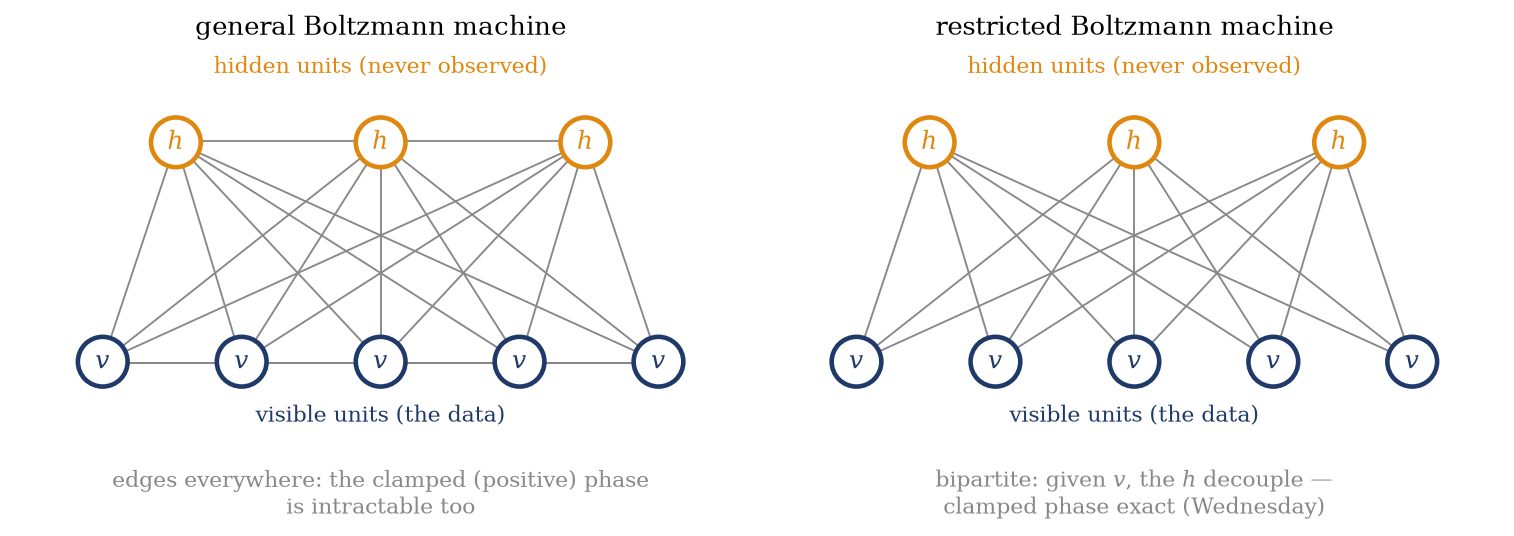
\[ \frac{\partial L}{\partial W_{ij}} \;=\; \langle v_i h_j \rangle_\text{clamped} \;-\; \langle v_i h_j \rangle_\text{model}, \]

with the derivation identical in structure to Section 5.4 — but read the first bracket carefully, because something just got worse. The hidden units are never observed, so the positive phase is no longer a lookup: it clamps the visibles to each data point and averages over the conditional \(p(h \mid v)\) — an inference problem inside the learning loop. For a general graph (Figure 5.4, left), that conditional couples all the hidden units to each other, and is itself intractable. Hidden units thus add a second hard expectation on top of the \(Z\) wall — and, as flagged in Section 5.4, they break the concavity of the objective as well.

Figure 5.4: Hidden units, and the restriction that will save the positive phase. Left: a general Boltzmann machine — visible units (data) and hidden units (latent), undirected couplings everywhere, including within each layer; the clamped conditional \(p(h \mid v)\) couples the hidden units to each other and is intractable. Right: the *restricted* Boltzmann machine — couplings only *between* the layers. Given the visibles, the hidden units decouple, the clamped (positive) phase factorizes exactly, and a whole layer can be sampled in parallel. The bipartite restriction and what it buys are the next lecture’s subject.

Two problems, two escapes — and they are exactly the next lecture’s program, so we name them and stop. ① Make the positive phase exact by architecture: forbid within-layer couplings, so that given \(v\) the hidden units decouple and \(p(h \mid v)\) factorizes — the restricted Boltzmann machine (Figure 5.4, right). ② Make the negative phase cheap by approximation: replace the equilibrated model average with a short Gibbs chain started at the data — contrastive divergence (Hinton 2002). Why a deliberately unconverged chain gives a usable gradient is a genuinely good question, and it is the next lecture’s; the tutorial will make you crack it on paper.

Take-home 3

Hidden units buy expressive power — marginalizing latents induces effective interactions of all orders among the visibles — at the price of a second hard expectation: the clamped positive phase \(\langle \cdot \rangle_{p(h \mid v)}\), intractable for a general graph (and concavity is lost). The bipartite restriction (RBM) makes the clamped phase exact; contrastive divergence makes the negative phase cheap; both are covered in the next lecture. \(Z\) itself remains standing, for Module 4.

5.7 Example: the \(Z\) ledger

One concrete machine, the negative phase computed exactly — then scaled until it breaks. Take \(N = 3\) spins, couplings \(J_{12} = J_{23} = 0.5\), \(J_{13} = -0.5\), biases \(\theta = 0\) — the machine already running in Figure 5.3. The product of couplings around the triangle is negative, so the loop is frustrated — no configuration can satisfy all three bonds at once (satisfying all three would cost \(E = -1.5\); the true ground states make do with \(-0.5\)). The negative phase asks for \(\langle s_1 s_2 \rangle_\text{model}\), and at \(N = 3\) we simply enumerate all \(2^3 = 8\) configurations:

\(s_1\, s_2\, s_3\)	\(E(s)\)	\(e^{-E}\)	\(s_1 s_2\, e^{-E}\)
\(+\,+\,+\)	\(-0.5\)	\(1.649\)	\(+1.649\)
\(+\,+\,-\)	\(-0.5\)	\(1.649\)	\(+1.649\)
\(+\,-\,+\)	\(+1.5\)	\(0.223\)	\(-0.223\)
\(+\,-\,-\)	\(-0.5\)	\(1.649\)	\(-1.649\)
\(-\,+\,+\)	\(-0.5\)	\(1.649\)	\(-1.649\)
\(-\,+\,-\)	\(+1.5\)	\(0.223\)	\(-0.223\)
\(-\,-\,+\)	\(-0.5\)	\(1.649\)	\(+1.649\)
\(-\,-\,-\)	\(-0.5\)	\(1.649\)	\(+1.649\)

Six degenerate low-energy states — the frustrated loop’s signature, and Week 2’s rugged-landscape story in miniature — and two high-energy ones. Summing the columns: \(Z = 6\, e^{0.5} + 2\, e^{-1.5} = 10.34\), and

\[ \langle s_1 s_2 \rangle_\text{model} \;=\; \frac{2.851}{10.34} \;=\; 0.276 \]

— the number the Glauber chain of Figure 5.3 was hunting. The negative phase is a completely well-defined, completely mechanical sum: eight energies, eight exponentials, one division. If the data were to report, say, \(\langle s_1 s_2 \rangle_\text{data} = 0.50\), the learning rule Equation 5.4 says \(\partial L / \partial J_{12} = 0.50 - 0.276 = +0.224\): strengthen the coupling, re-enumerate, repeat. Nothing about the rule is hard.

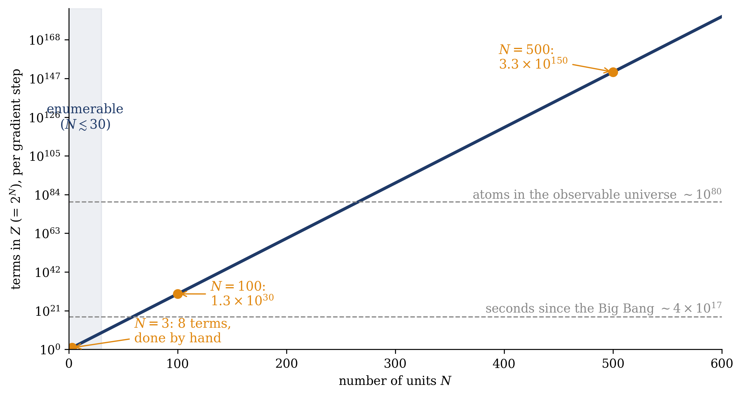
Now scale it. The number of terms in \(Z\) — and in every negative-phase expectation, at every gradient step — is \(2^N\):

\(N\)	\(2^N\) terms in \(Z\)	feasibility
\(3\)	\(8\)	done by hand above
\(10\)	\(1{,}024\)	a laptop, instantly
\(20\)	\(\sim 1.05 \times 10^{6}\)	a laptop, seconds
\(30\)	\(\sim 1.07 \times 10^{9}\)	a memory-bound minute — the practical ceiling for brute force
\(100\)	\(\sim 1.27 \times 10^{30}\)	more terms than seconds since the Big Bang (\(\sim 4 \times 10^{17}\))
\(500\)	\(\sim 3.3 \times 10^{150}\)	more terms than atoms in the observable universe (\(\sim 10^{80}\))

The last two rows set the scale. A machine of \(100\) units — not a large model; a thumbnail image — asks, for its exact negative phase, for more terms than there have been seconds since the Big Bang. At \(500\) units the count dwarfs the atom inventory of the observable universe. And this is not a one-time cost: the trap of Section 5.5 says the sum is owed per gradient step, because the distribution under the bracket moves with the parameters. Figure 5.5 draws the scaling.

Show code

N = np.arange(1, 601)
fig, ax = plt.subplots(figsize=(8.6, 4.6))
ax.semilogy(N, 2.0**N, color=NAVY, lw=2.5)
ax.axvspan(0, 30, color=NAVY, alpha=0.08)
ax.text(15, 1e120, "enumerable\n($N \\lesssim 30$)", color=NAVY, fontsize=10.5, ha="center")
ax.axhline(4.4e17, color=GRAY, ls="--", lw=1)
ax.text(600, 1.5e18, "seconds since the Big Bang $\\sim 4\\times 10^{17}$",
        color=GRAY, fontsize=10, ha="right", va="bottom")
ax.axhline(1e80, color=GRAY, ls="--", lw=1)
ax.text(600, 3e80, "atoms in the observable universe $\\sim 10^{80}$",
        color=GRAY, fontsize=10, ha="right", va="bottom")
for n, lab, xy in [(3, "$N=3$: 8 terms,\ndone by hand", (60, 1e4)),
                   (100, "$N=100$:\n$1.3\\times 10^{30}$", (130, 1e24)),
                   (500, "$N=500$:\n$3.3\\times 10^{150}$", (395, 3e152))]:
    ax.plot([n], [2.0**n], "o", color=ORANGE, ms=7)
    ax.annotate(lab, xy=(n, 2.0**n), xytext=xy, color=ORANGE, fontsize=10.5,
                arrowprops=dict(arrowstyle="->", color=ORANGE, lw=1))
ax.set_xlabel(r"number of units $N$")
ax.set_ylabel(r"terms in $Z$ (= $2^N$), per gradient step")
ax.set_xlim(0, 600); ax.set_ylim(1, 1e185)
fig.tight_layout(); plt.show()

Figure 5.5: The \(Z\) wall: the number of terms in the partition function — and in every exact negative-phase expectation, at every gradient step — against the number of units \(N\). Exhaustive enumeration is comfortable in the shaded region below \(N \approx 30\) and hopeless beyond: by \(N = 100\) the sum has more terms than seconds since the Big Bang (\(\sim 4 \times 10^{17}\)), by \(N = 500\) more than atoms in the observable universe (\(\sim 10^{80}\)). The learning rule Equation 5.4 is one line; the negative phase inside it is this curve. The rest of the course is strategies for the region right of the shading.

Learning is easy where you average over data and impossible where you average over the model — and that gap is the partition function.

The warm-up card (due the evening before the next lecture, with the Hinton reading) puts you at this wall deliberately: a tiny machine with hidden units, \(Z\) computed by hand, then scaled up until it breaks — the ledger above, with the hidden-unit sum of Section 5.6 layered on top. The workaround arrives in the next lecture; for now the obstruction stands on its own.

5.8 Outlook: two escapes, and a far arrow

We heated Week 2’s network and recovered Week 1’s distribution — the course’s two opening moves now joined in one machine. We asked that machine to learn and obtained a physically transparent learning rule: data correlations minus model correlations, wake minus sleep. And we derived, rather than asserted, why that rule cannot be run as written: its second term is \(\nabla_\theta \log Z\), an exponentially large sum, owed anew at every step — with a second difficulty, mixing, standing behind the first. The practitioner’s summary: an energy-based model is easy to write down and intractable to normalize, and every training algorithm you will meet from here on is a strategy for the negative phase.

The next lecture addresses the wall in two moves already named: the bipartite restriction that makes the clamped phase exact and lets whole layers sample in parallel, and contrastive divergence — a deliberately short, deliberately biased chain started at the data (Hinton 2002) — with the good question of why a truncated chain is allowed at its center. The tutorial works through the RBM gradient, identifying and evading the \(Z\)-term.

One forward pointer, now precise. The negative phase exists because we differentiate \(\log Z\) with respect to the parameters: \(\nabla_\theta \log Z = \langle \cdot \rangle_\text{model} \neq 0\). In Week 10, score matching will fit the very same unnormalized energies by working instead with the gradient with respect to the configuration — and there \(\nabla_x \log Z = 0\), identically, because \(Z\) does not depend on where you evaluate the density (Hyvärinen 2005). The claim is precise: \(Z\) is not made zero — a different derivative of it is zero, and shifting the derivative from \(\theta\) to \(x\) without losing the ability to learn is the whole trick. The derivation comes in Week 10.