8 The modern Hopfield network: attention is memory

8.1 Two titles, one claim

The previous lecture ended on a deliberately unresolved gesture: make the states continuous, and the retrieval rule collapses to a single step — a rule you will recognize. This lecture delivers the identification.

In 2017, Vaswani and coauthors announced to machine learning that Attention Is All You Need (Vaswani et al. 2017) — and the transformer architecture built on that paper came to dominate the entire field: language, vision, protein structure, code. In 2021, Ramsauer and coauthors — Hochreiter’s group in Linz — replied with a paper called Hopfield Networks is All You Need (Ramsauer et al. 2021). The two titles are one claim. The attention mechanism at the center of modern AI is the retrieval update of a continuous Hopfield network — Week 2’s machine, scaled by the previous lecture’s dial and made smooth, written in an engineer’s notation. (Attention entered machine learning as a learned alignment for machine translation (Bahdanau, Cho, and Bengio 2015); nobody involved was thinking about spin systems. The identification came after the architecture had taken over, making it a discovery about structure, not a design choice.)

An attention layer is one step of energy descent in an associative memory — a differentiable, content-addressable lookup, the direct continuous descendant of Hopfield (1982). Far from being a historical curiosity capped at \(0.138\,N\), the energy-based view of computation — scaled (the previous lecture) and made continuous (today) — is the mechanism at the heart of the architecture that now dominates machine learning. Today’s normalizer is a softmax denominator over a finite set of stored patterns, Week 1’s tractable case; \(Z\) remains absent. Module 2, which requires normalized distributions, reintroduces it.

Take-home 1

Attention Is All You Need and Hopfield Networks is All You Need are the same claim. A transformer attention layer is one step of retrieval in a continuous modern Hopfield network — content-addressable memory, written in ML notation.

8.2 From hard max to soft max

Two objects that look unrelated — a physicist’s associative memory (an energy over states, minimized to retrieve a stored pattern from a cue) and an ML engineer’s attention layer (a query, a stack of keys and values, a softmax-weighted readout) — will each be built from its own side and then set on the same line. Both share a single picture: a query vector reaching into a cloud of stored patterns, a weight on each pattern proportional to how well it matches, and an output assembled as the weighted sum. The sections below construct the picture from each side and identify them.

A single substitution separates the previous lecture’s network from the continuous version. The previous lecture’s exponential interaction made the effective field a filter, \(F' = e^{\text{overlap}}\), which in the sharp limit selects the best-matching pattern — a hard \(\max\) over overlaps. Two things are wrong with a hard \(\max\) if you want to build it into a neural network: it is not differentiable (no gradients can flow through it), and the previous lecture’s retrieval still ran by discrete spin flips, many of them. The fix is one of applied mathematics’ oldest moves — replace the max by its smooth version:

\[ \operatorname{lse}(\beta, z) \;=\; \frac{1}{\beta} \log \sum_{\mu=1}^{M} e^{\beta z_\mu}, \qquad \nabla_z \operatorname{lse}(\beta, z) \;=\; \operatorname{softmax}(\beta z), \]

log-sum-exp: the smooth max; softmax: the smooth argmax

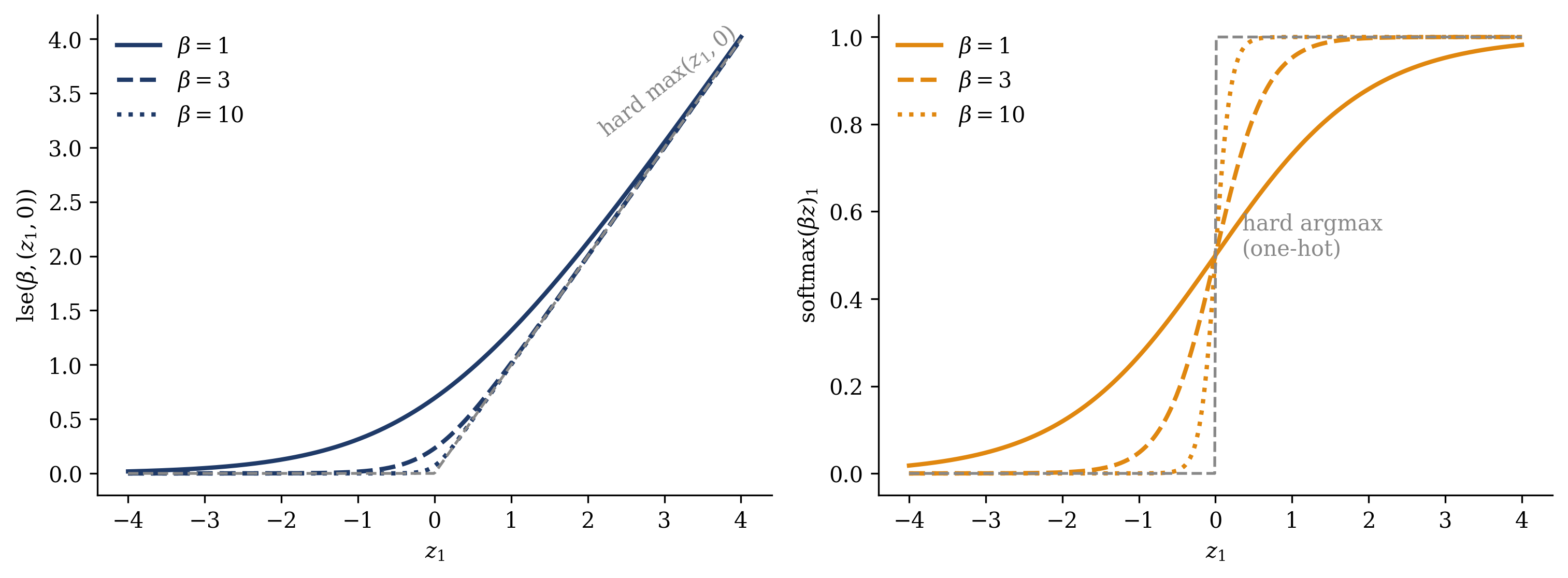
the log-sum-exp, whose gradient is the softmax. As \(\beta \to \infty\), \(\operatorname{lse} \to \max\) and \(\operatorname{softmax} \to\) the one-hot \(\operatorname{argmax}\): the previous lecture’s hard selection recovered. At finite \(\beta\), both are smooth, differentiable, and therefore trainable. Figure 8.1 draws the pair. Two familiar objects appear here: for two options, \(\operatorname{lse}\) is the softplus of Section 6.3 — the RBM’s traced-out hidden unit was a two-state log-sum-exp all along — and the softmax is Week 1’s Boltzmann distribution over a finite menu (Section 1.6), which is precisely why \(Z\) poses no problem today.

Show code

z = np.linspace(-4, 4, 400)
fig, (a1, a2) = plt.subplots(1, 2, figsize=(10.2, 3.8))
for beta, ls in zip([1, 3, 10], ["-", "--", ":"]):
    a1.plot(z, np.log1p(np.exp(beta * z)) / beta, color=NAVY, ls=ls, lw=2,
            label=rf"$\beta = {beta}$")
    a2.plot(z, 1 / (1 + np.exp(-beta * z)), color=ORANGE, ls=ls, lw=2,
            label=rf"$\beta = {beta}$")
a1.plot(z, np.maximum(z, 0), color=GRAY, ls="--", lw=1.3)
a1.text(2.1, 3.1, r"hard $\max(z_1, 0)$", color=GRAY, fontsize=10, rotation=38)
a1.set_xlabel(r"$z_1$"); a1.set_ylabel(r"$\operatorname{lse}(\beta, (z_1, 0))$")
a1.legend(frameon=False, fontsize=10, loc="upper left")
a2.plot(z, (z > 0).astype(float), color=GRAY, ls="--", lw=1.3)
a2.text(0.35, 0.5, "hard argmax\n(one-hot)", color=GRAY, fontsize=10)
a2.set_xlabel(r"$z_1$"); a2.set_ylabel(r"$\operatorname{softmax}(\beta z)_1$")
a2.legend(frameon=False, fontsize=10, loc="upper left")
fig.tight_layout(); plt.show()

Figure 8.1: The smooth max and the smooth argmax, drawn for two options \(z = (z_1, 0)\). Left: \(\operatorname{lse}(\beta, z) = \beta^{-1}\log(e^{\beta z_1} + 1)\) approaches the hard \(\max(z_1, 0)\) (dashed) as \(\beta\) grows — and the \(\beta = 1\) curve is exactly the softplus that appeared when Week 3 traced out an RBM’s hidden unit. Right: the corresponding weight \(\operatorname{softmax}(\beta z)_1 = \sigma(\beta z_1)\) sharpens from a gentle preference to the hard one-hot \(\operatorname{argmax}\) (dashed step). The continuous modern Hopfield network is the previous lecture’s hard pattern-selection with these smooth versions substituted — differentiable, one-step, trainable — and \(\beta\) sets how close to hard.

Three steps remain: ① the energy whose minimization performs this soft selection; ② its one-step update; ③ the identification of that update with attention.

8.3 The engine: the log-sum-exp energy and its one-step update

Setup. Stack the \(M\) stored patterns as the columns of a matrix, \(X = [\,x_1, \dots, x_M\,]\), each \(x_\mu \in \mathbb{R}^d\) — continuous vectors now, not spins. The state is a continuous query \(\xi \in \mathbb{R}^d\), and \(\beta > 0\) is an inverse temperature. (A notation flag, since we adopt Ramsauer’s: through Weeks 2–4 the symbol \(\xi^\mu\) was a stored pattern and the count was \(P\); from here \(\xi\) is the query state, the stored patterns are the \(x_\mu\), and their number is \(M\) — the relabeling brings us into line with the attention literature we are about to meet.) Following Ramsauer et al. (2021), take the smooth max of the overlaps as the attracting part of the energy, and add a quadratic to keep it bounded below:

\[ E(\xi) \;=\; -\operatorname{lse}\big(\beta,\, X^T \xi\big) \;+\; \tfrac{1}{2}\, \xi^T \xi \;+\; \text{const} \tag{8.1}\]

continuous modern Hopfield energy

(The constant, \(\beta^{-1}\log M + \tfrac{1}{2} M_\text{max}^2\) with \(M_\text{max}\) the largest pattern norm, makes \(E \geq 0\); it carries no \(\xi\)-dependence and will not survive a gradient, so we drop it from every display that follows.) Before differentiating, consider the landscape: \(-\operatorname{lse}\) digs a well wherever \(\xi\) has a large overlap with some stored pattern — one well per pattern, deeper and narrower as \(\beta\) sharpens — and the quadratic term is the bowl that keeps a query from running off to infinity along a pattern direction. This is the previous lecture’s picture (Figure 7.1, right panel), drawn in a continuous space.

The gradient, in full. The computation is the chain rule. Component \(i\):

\[ \frac{\partial}{\partial \xi_i} \operatorname{lse}\big(\beta, X^T \xi\big) \;=\; \frac{1}{\beta}\, \frac{\sum_\mu \beta\, x_{\mu i}\, e^{\beta\, x_\mu \cdot \xi}}{\sum_\nu e^{\beta\, x_\nu \cdot \xi}} \;=\; \sum_\mu x_{\mu i} \underbrace{\frac{e^{\beta\, x_\mu \cdot \xi}}{\sum_\nu e^{\beta\, x_\nu \cdot \xi}}}_{=\;\operatorname{softmax}\left(\beta X^T \xi\right)_\mu}, \]

or, assembled over components,

\[ \nabla_\xi \operatorname{lse}\big(\beta, X^T \xi\big) \;=\; X\, \operatorname{softmax}\big(\beta X^T \xi\big), \qquad\Longrightarrow\qquad \nabla_\xi E \;=\; \xi \;-\; X\, \operatorname{softmax}\big(\beta X^T \xi\big). \]

The stationary condition is the update. Set \(\nabla_\xi E = 0\):

\[ \boxed{\; \xi^\text{new} \;=\; X\, \operatorname{softmax}\big(\beta\, X^T \xi\big) \;} \tag{8.2}\]

one-step retrieval update

In words: the retrieved state is a softmax-weighted average of the stored patterns, each weighted by how well it matches the current query. This is the previous lecture’s \(F'\)-filter made smooth — score every memory against the cue, exponentiate, normalize, and blend — with softmax playing the role of “select the matching pattern,” softly.

Three properties make this equation a usable neural-network layer.

First, iterating the update descends the energy. The energy Equation 8.1 splits by construction into a concave piece (\(-\operatorname{lse}\); the log-sum-exp is convex, so its negative is concave) plus a convex piece (\(\tfrac12\|\xi\|^2\)). For exactly such splittings, the concave–convex procedure of Yuille and Rangarajan (2003) supplies a descent scheme: at the current point, replace the concave piece by its tangent plane — which, by concavity, lies above it everywhere — and minimize the resulting convex upper bound exactly. Minimizing \(\tfrac12\|\xi\|^2\) minus the linearization \(\big(X\operatorname{softmax}(\beta X^T\xi^t)\big)\!\cdot\xi\) is a one-line quadratic problem, and its solution is precisely Equation 8.2. Each iterate therefore minimizes a surface that touches \(E\) at the current point and majorizes it elsewhere, so \(E\) can only decrease: the Lyapunov property of Section 3.4, in its third incarnation — discrete flips (W2), Glauber’s stochastic flips (W3), and now a smooth map.

Second, one step is essentially enough. Ramsauer et al. (2021) quantify what “well-separated” buys: define a pattern’s separation \(\Delta_\mu\) as the gap between its self-overlap and its largest rival overlap, \(\Delta_\mu = x_\mu \cdot x_\mu - \max_{\nu \neq \mu} x_\mu \cdot x_\nu\). For \(\Delta_\mu\) sufficiently large (relative to \(1/\beta\)), the update is a contraction near \(x_\mu\), a fixed point exists exponentially close to the pattern, and — the key consequence for practice — a single application of Equation 8.2 starting anywhere in the basin lands exponentially close to that fixed point. Retrieval is not Week 2’s long relaxation of single-spin flips; it is one differentiable map, evaluated once — which is exactly the property that lets it sit as a layer inside a network trained end-to-end by backpropagation.

Third, the storage matches the previous lecture’s. The number of random patterns (say, placed on the sphere) that remain well-separated in the above sense — and hence individually retrievable — grows exponentially with the dimension \(d\) (Ramsauer et al. 2021): the continuous network inherits the exponential capacity of the \(F = e^x\) interaction it descends from, with \(d\) playing the role the previous lecture’s \(N\) played. (For the unified view of why the inheritance is exact — discrete and continuous networks as two choices of “Lagrangian” in one general framework, with the update rules and energies generated mechanically from that choice — see Krotov and Hopfield (2021), the general treatment behind both of this week’s lectures; a script-level pointer, not an examinable one.)

The inverse temperature \(\beta\) controls the behavior. Large \(\beta\): the softmax approaches a one-hot vector, and the update returns the single nearest pattern — exact retrieval, the previous lecture’s sharp limit. Small \(\beta\): the softmax spreads, and the update returns a broad weighted average of several patterns — the previous lecture’s metastable mixtures, now produced deliberately. One parameter sweeps from lookup to blending; in the next section it acquires a famous name.

8.4 This update is attention

The update, read as an engineer would, is a matrix, a softmax, and a matrix — the structure of transformer attention.

Recall, from the companion course, the equation at the center of the transformer (Vaswani et al. 2017). Given a stack of queries \(Q\) (one per row), keys \(K\), and values \(V\) (one per row), scaled dot-product attention computes

\[ \operatorname{Attention}(Q, K, V) \;=\; \operatorname{softmax}\!\Big( \frac{Q K^T}{\sqrt{d_k}} \Big)\, V . \]

Take our update Equation 8.2, transpose it into the same row-vector convention (a query is a row \(q = \xi^T\); the stored patterns are the rows of \(X^T\)), and it reads \(q^\text{new} = \operatorname{softmax}\big(\beta\, q\, (X^T)^T\big)\, X^T\). Set the two equations on one line:

\[ q^\text{new} = \operatorname{softmax}\big(\beta\, q K^T\big)\, V \qquad\longleftrightarrow\qquad \operatorname{softmax}\!\Big( \frac{Q K^T}{\sqrt{d_k}} \Big)\, V, \]

and read off the dictionary:

\[ \boxed{\; Q \leftrightarrow \text{the query state } \xi, \qquad K \leftrightarrow \text{the stored patterns (keys)}, \qquad V \leftrightarrow \text{the stored patterns (values)}, \qquad \beta \leftrightarrow \frac{1}{\sqrt{d_k}}. \;} \tag{8.3}\]

attention = one step of Hopfield retrieval

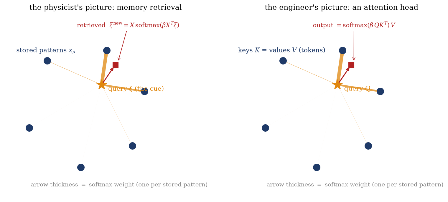
One transformer attention layer is one step of modern Hopfield retrieval. The queries are cues; the keys are the stored patterns the cue is matched against; the values are the stored patterns that get blended into the output; and \(1/\sqrt{d_k}\) is the inverse temperature of the lookup. Figure 8.2 draws the identification: one picture, computed once, labeled twice.

For the record — the tutorial develops it at the board, and the script mirrors it here — the dressed dictionary, as transformers actually implement it. The correspondence above is the skeleton (\(K = V = X\), no learned parameters); a real attention layer inserts three linear maps: \(Q = \Xi\, W_Q\), \(K = Y\, W_K\), \(V = Y\, W_V\), where \(\Xi\) holds the querying tokens and \(Y\) the attended-to tokens. Read as memory, the projections are natural rather than decorative: \(W_K\) chooses in which learned subspace the matching is scored (what counts as similar), \(W_V\) chooses what is returned when a pattern matches (the payload need not be the address), and \(W_Q\) maps the current token into the matching space — a content-addressable memory whose addressing scheme and stored content are themselves learned. Self-attention is the case \(Y = \Xi\): the sequence is its own memory, every token a query into all the others. Cross-attention stores one sequence and queries it with another — an encoder’s output retrieved by a decoder, which is exactly the alignment problem attention was invented for (Bahdanau, Cho, and Bengio 2015). Multi-head attention runs \(h\) such retrievals in parallel, each with its own projections — \(h\) associative memories reading the same tokens through different learned lenses, their outputs concatenated — and stacking layers is not iterating one memory to convergence but taking single retrieval steps through a sequence of different learned memories, each one step deep.

Figure 8.2: One calculation, two labelings. A query reaches into a cloud of six stored patterns; each pattern receives a softmax weight (arrow thickness) according to its overlap with the query; the output is the weighted average, pulled toward the best-matching pattern. Left, the physicist’s labels: cue, stored patterns, retrieval \(\xi^\text{new} = X\operatorname{softmax}(\beta X^T\xi)\). Right, the engineer’s labels: query, keys and values, attention output \(\operatorname{softmax}(\beta\, QK^T)V\). The geometry, the weights, and the output are identical — the relabeling is the theorem.

The role of \(\sqrt{d_k}\). The scaling in Vaswani’s denominator is introduced, in the original paper, as a numerical fix: dot products of \(d_k\)-dimensional vectors with \(\mathcal{O}(1)\) components grow like \(\sqrt{d_k}\), and without the division the softmax saturates — one weight near \(1\), the rest near \(0\), gradients vanishing through the flat tails. Read through today’s dictionary, that fix is a temperature: \(\beta = 1/\sqrt{d_k}\) holds the retrieval at moderate sharpness as the dimension grows, deliberately keeping attention out of the hard-argmax regime. This is a statistical-mechanics temperature inside a normalization constant from Vaswani et al. (2017), made explicit four years later by the Hopfield reading (Ramsauer et al. 2021) — and note the direction of the effect, because it is easy to read backwards: larger \(d_k\) means smaller \(\beta\), hence a softer, more-averaging lookup. The \(\sqrt{d_k}\) prevents over-sharpening; it does not sharpen.

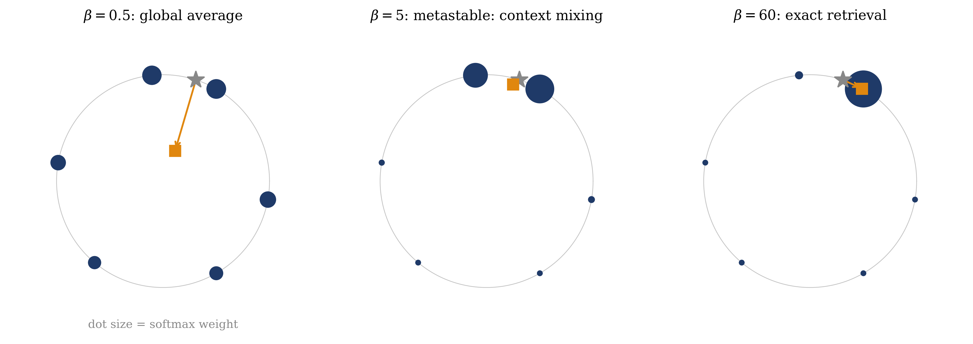
Metastable states as a feature. The previous lecture’s mixture states — retrievals that blend several nearby patterns — were discussed as a cost of the exponential interaction. For an attention head they are the desired output: a query (a token in context) rarely wants a single stored pattern; it wants a weighted blend of everything relevant — several previous tokens, in proportion to their relevance. That is precisely a metastable average, produced on purpose at moderate \(\beta\). The defect of an exact memory is the mechanism of a context-mixer, and the transformer’s own temperature choice parks it deliberately in the mixing regime. Figure 8.3 runs the three regimes on one query.

Show code

ang = np.deg2rad([60, 96, 170, 230, 300, 350])
Xp = np.c_[np.cos(ang), np.sin(ang)]                       # patterns as rows
q = np.array([np.cos(np.deg2rad(72)), np.sin(np.deg2rad(72))])
fig, axes = plt.subplots(1, 3, figsize=(11.4, 3.9))
titles = ["global average", "metastable: context mixing", "exact retrieval"]
for ax, beta, ttl in zip(axes, [0.5, 5, 60], titles):
    w = np.exp(beta * Xp @ q); w /= w.sum()
    out = w @ Xp
    th = np.linspace(0, 2 * np.pi, 200)
    ax.plot(np.cos(th), np.sin(th), color=GRAY, lw=0.6, alpha=0.5)
    ax.scatter(Xp[:, 0], Xp[:, 1], s=900 * w + 15, color=NAVY, zorder=3)
    ax.plot([q[0]], [q[1]], "*", color=GRAY, ms=15, zorder=4)
    ax.plot([out[0]], [out[1]], "s", color=ORANGE, ms=9, zorder=4)
    ax.annotate("", xy=(out[0], out[1]), xytext=(q[0], q[1]),
                arrowprops=dict(arrowstyle="->", color=ORANGE, lw=1.5))
    ax.set_title(rf"$\beta = {beta}$: {ttl}", fontsize=11.5)
    ax.set_xlim(-1.45, 1.45); ax.set_ylim(-1.45, 1.45)
    ax.set_aspect("equal"); ax.axis("off")
axes[0].text(0, -1.38, "dot size = softmax weight", color=GRAY,
             fontsize=9.5, ha="center")
fig.tight_layout(); plt.show()

Figure 8.3: The three retrieval regimes of the one-step update Equation 8.2, computed exactly for a query (star) amid six stored patterns (dots, sized by their softmax weight; the orange square is the retrieved \(\xi^\text{new}\)). Two of the patterns are deliberately close, and the query sits near both. Left, \(\beta = 0.5\): weights nearly uniform — the update returns a global average, useless as memory. Center, \(\beta = 5\): the weight concentrates on the two matching patterns (\(w \approx 0.57\) and \(0.42\)) — a *metastable* average, blending exactly the relevant items: this is what an attention head does to its context, and where \(\beta = 1/\sqrt{d_k}\) deliberately operates. Right, \(\beta = 60\): one-hot weights — exact single-pattern retrieval, the previous lecture’s sharp limit.

Two caveats, to state the equivalence precisely. First, one layer is one step: a transformer does not iterate Equation 8.2 to a fixed point — it takes a single retrieval step per attention layer and stacks layers, each with its own learned memory. “Attention minimizes an energy” overclaims; attention takes one descent step on an energy is the theorem. Second, the softmax denominator here — the sum over the \(M\) stored patterns or tokens — is a partition function over a finite menu, Week 1’s tractable case (Section 1.6), not the \(2^N\) configuration sum of Week 3. \(Z\) is genuinely absent from every transformer forward pass; do not import Week 3’s obstruction into a lookup that does not have it.

Trap

Two readings that are wrong in opposite directions. ① \(\beta = 1/\sqrt{d_k}\) means larger key dimension gives a softer, more-averaging attention — the scaling exists to prevent softmax saturation, not to sharpen the lookup. ② One attention layer performs one retrieval step, not a relaxation to a fixed point; and in a trained transformer \(K \neq V\) in general (separate learned projections of the same tokens). The equivalence is exact about structure and about one step — claim neither more nor less.

Take-home 2

Transformer attention \(\operatorname{softmax}(QK^T/\sqrt{d_k})\,V\) is the one-step modern Hopfield update \(X\operatorname{softmax}(\beta X^T\xi)\): query = cue, keys = values = stored patterns (learned projections in general), \(\beta = 1/\sqrt{d_k}\). The \(\sqrt{d_k}\) is a retrieval temperature that keeps attention in the soft regime; metastable averaging is context-mixing. Attention is content-addressable memory.

8.5 Example: one calculation, two names

One small memory, the update computed by hand, and the same numbers read twice. Store \(M = 4\) patterns in \(d = 3\): the unit vectors \(x_1 = (1,0,0)\), \(x_2 = (0,1,0)\), \(x_3 = (0,0,1)\), and the blend \(x_4 = (0, 1, 1)/\sqrt{2}\). The query is a corrupted version of the first memory, leaning toward the second: \(\xi = 0.8\, x_1 + 0.2\, x_2\), with overlaps \(X^T\xi = (0.8,\ 0.2,\ 0,\ 0.14)\). Compute \(w = \operatorname{softmax}(\beta X^T \xi)\) and \(\xi^\text{new} = Xw\) at three temperatures:

regime	\(\beta\)	weights \(w\)	\(\xi^\text{new}\)	reading
soft	\(1/\sqrt{3} \approx 0.58\)	\((0.33,\ 0.23,\ 0.21,\ 0.23)\)	\((0.33,\ 0.39,\ 0.37)\)	global average — everything blended
moderate	\(3\)	\((0.72,\ 0.12,\ 0.07,\ 0.10)\)	\((0.72,\ 0.19,\ 0.14)\)	metastable: \(x_1\) dominant, context mixed in
sharp	\(20\)	\((1.00,\ 0.00,\ 0.00,\ 0.00)\)	\((1.00,\ 0.00,\ 0.00) = x_1\)	exact retrieval — the previous lecture’s hard limit

The three rows illustrate the full range: at \(\beta = 20\) the memory returns its first pattern exactly (the weight on \(x_1\) is \(0.99999\)); at \(\beta = 3\) it returns “mostly \(x_1\), with the relevant neighbors mixed in”; at \(\beta = 0.58\) it returns an undifferentiated average of everything. Now read the first row’s temperature again: \(1/\sqrt{3}\) is precisely the transformer’s own \(\beta = 1/\sqrt{d_k}\) for \(d_k = 3\). On this toy the engineer’s default temperature sits deep in the averaging regime — by design, and (in a real transformer) with learned projections rescaling the logits to taste around it.

The second reading makes the identification explicit. Set \(Q = \xi\) as a row, \(K = V =\) the patterns as rows, \(d_k = 3\); then \(\operatorname{softmax}(QK^T/\sqrt{d_k})\,V\) is — symbol for symbol — the first row of the table. The physicist retrieved a memory at soft temperature; the engineer computed an attention head; the arithmetic was identical. The calculation is one; only the labels differ.

The tutorial (16–18, Ph12 106) is derivation-led: both equations, from both fields, are set side by side — deriving attention from the Hopfield side and Hopfield from the attention side, then building out the full dictionary: separate \(W_Q, W_K, W_V\) projections, self- versus cross-attention, and multi-head attention as parallel associative memories.

A transformer attention layer is one step of Hopfield retrieval — attention is associative memory.

8.6 Module 1 closes: the landscape, all the way up

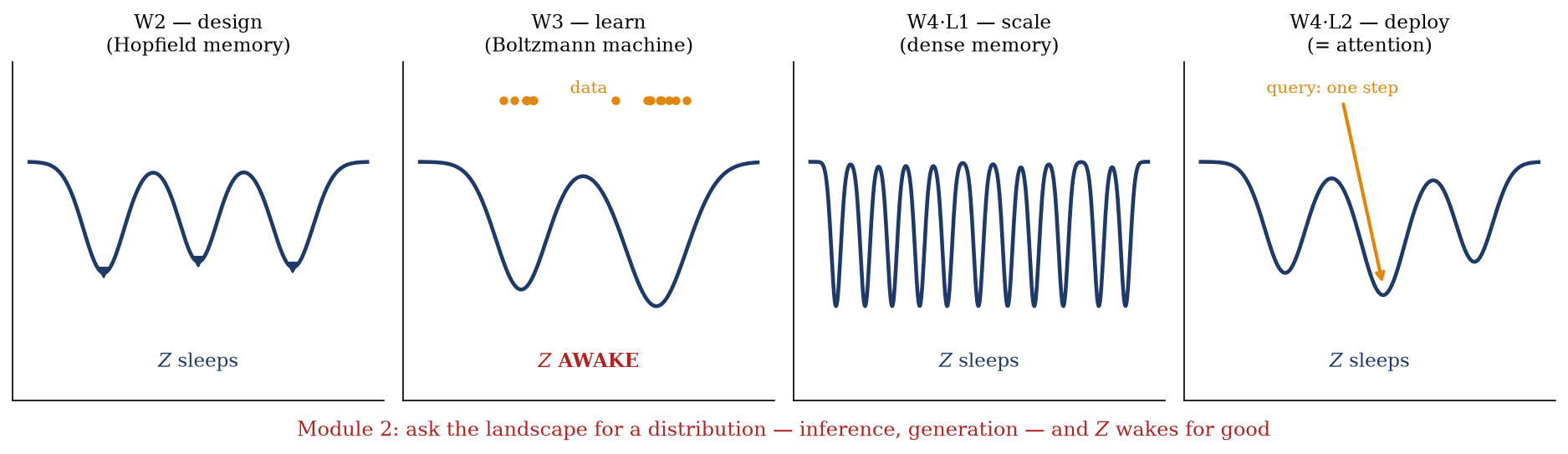
Four weeks ago we drew an energy landscape over configuration space. Week 2 designed the landscape: Hopfield’s memory, minima placed at data by Hebb’s rule, retrieval as descent — a machine that computes, capped at \(0.138\,N\), with nothing normalized and no \(Z\) in sight. Week 3 learned the landscape: heat the network and it becomes a probability model; fit its couplings by maximum likelihood and the gradient sprouts \(\nabla_\theta \log Z\) — a sum over \(2^N\) states, dodged but not defeated by contrastive divergence. The previous lecture scaled the landscape: the interaction function turned out to be a capacity dial, and the wall at \(138\) patterns moved past the atom count of the universe. And today the landscape deployed: made continuous and smooth, its one-step retrieval is the attention layer — the mechanism running inside essentially every large model in existence. Figure 8.4 draws the four panels in a row, with the role of \(Z\) marked week by week.

Figure 8.4: Module 1 in four panels — one landscape, four verbs. Week 2 *designs* it (memory basins, nothing normalized); Week 3 *learns* it (basins molded under data, and the partition function enters as the training obstruction); Week 4 *scales* it (dense memory, exponentially many wells) and *deploys* it (a query descending in one step: attention). The pattern is the module’s lesson: \(Z\) is absent whenever the landscape only *retrieves*, and returns whenever the landscape must carry a normalized *distribution* — which is Module 2’s opening condition.

Deep learning’s central mechanism is itself energy-based. Hopfield’s 1982 landscape and Vaswani’s 2017 attention are one picture, thirty-five years apart, and the 2024 Nobel’s two halves — the memory and the learning machine — meet in Equation 8.3.

\(Z\) was absent in Week 2 (\(T = 0\), nothing normalized), central in Week 3 (learning a distribution), and absent again all through Week 4 (finite normalizers — a softmax over patterns, never a sum over configurations). The pattern is exact: whenever the landscape only retrieves, \(Z\) plays no role; whenever the landscape must carry a normalized distribution, \(Z\) returns. Module 2 asks for distributions everywhere — inference over hidden variables, marginals of rugged systems, generative modeling proper — so from next week \(Z\) is present throughout, and the response changes character, from Week 3’s dodge to the first principled approximation of the distribution itself. Week 5 builds mean-field theory and the variational free energy — the Gibbs–Bogoliubov bound that turns “compute \(\log Z\)” into “optimize over tractable families”; Week 6 sharpens it (TAP corrections, belief propagation); Week 7 carries it to latent-variable models and the variational autoencoder. And behind all of it stands, unchanged, the far promise this module made precise: what Module 2 approximates and Module 3 samples, Week 10 dissolves — \(\nabla_x \log Z = 0\), the derivative that is zero because it moves the configuration and not the parameters.

Take-home 3 — the Module 1 capstone

Module 1 in one line: the energy landscape — designed (W2), learned (W3), scaled and deployed (W4) — is the substrate of modern generative AI, and transformer attention is its retrieval step. The recurring obstruction is \(Z\), which appears exactly when the landscape must carry a normalized distribution; taming it — by approximation (M2), by sampling (M3), by elimination (M4) — is the rest of the course.