Core (~1 h).Chaudhari et al. (2017) — entropy-SGD, the algorithm that turns this lecture’s thesis into a training objective: read §3–§4 for the local free energy and its inner sampler. Alongside it, Keskar et al. (2017) — the empirical anchor: large-batch training finds sharp minima that generalize worse; read for the evidence, especially the sharpness–gap plots.
Optional background.Hochreiter and Schmidhuber (1997) — Flat Minima, the original argument (via minimum description length), made twenty years before deep learning could test it. Hinton and Camp (1993) — the MDL/Bayesian ancestor: free energy as a complexity penalty on weights. MacKay (2003), Ch. 28 — the Occam factor done cleanly from the Bayesian side. Dinh et al. (2017) — the essential caveat, Sharp Minima Can Generalize for Deep Nets; read last, so the caveat lands on a formed picture.
Prerequisite reminder. All of the previous lecture — SGD samples \(e^{-L/T}\) (Equation 17.4) at temperature \(T \propto \eta/|B|\) (Equation 17.2), with anisotropic noise (Section 17.5); Laplace’s method Equation 2.2 and the Gaussian integral Equation 2.1 (Week 1); the free energy \(F = \langle E \rangle - TS\) (Week 1) and its career as an objective (Weeks 5 and 7, Equation 14.6); SGLD as the deliberate sampler (Welling and Teh 2011). New content: flat versus sharp minima, the Occam factor as basin entropy, SGD’s free-energy preference, and entropy-SGD.
18.1 Which minimum?
The previous lecture ended with training revealed as sampling: SGD draws from \(e^{-L/T}\), thermalizing around minima rather than reaching them. A question follows immediately. A modern network’s loss landscape holds astronomically many minima, and gradient training will find one of them — but the minima are not interchangeable. Two parameter vectors with the same training loss can differ substantially on test data; whatever separates them is invisible to the loss value itself. The empirical discriminator has been known, in outline, for a long time: flat minima generalize, sharp minima do not. A minimum sitting in a wide, low-curvature basin tolerates perturbation — including the perturbation that matters, the shift from the training loss to the test loss — while a needle-thin minimum of identical depth is brittle. Which basin the optimizer lands in therefore decides generalization, and the previous lecture’s thermodynamics decides which basin the optimizer lands in.
The history assembles across three decades. Hochreiter and Schmidhuber (1997) argued that flat minima generalize because they can be described cheaply — a minimum-description-length argument with Hinton and Camp (1993) as its ancestor, where the free energy of the weights is literally a complexity penalty; both are the Bayesian Occam’s razor of MacKay (2003), translated to network weights. Twenty years later Keskar et al. (2017) supplied the modern evidence: large-batch training — which the previous lecture taught us to read as low-temperature training — systematically finds sharper minima with worse test error. And Chaudhari et al. (2017) closed the loop by building the preference into an algorithm, entropy-SGD, whose objective is not the loss but a local free energy. That free energy is where the physics enters, and it is the same object this course has carried since Week 1.
The question: why do flat minima generalize, and why does SGD — untold about any of this — find them? A finite-temperature sampler does not seek the lowest energy but the lowest free energy, energy minus temperature times entropy; a basin’s entropy is the log of its volume; and a flat minimum is a high-entropy minimum. SGD is that sampler, by the previous lecture’s derivation, and its temperature \(\eta/|B|\) tunes how strongly volume competes with depth. Module 3 closes with the course’s central object applied to generalization.
Take-home 1
Minima with equal training loss can generalize very differently, and the discriminator is flatness: a wide basin is robust to the train→test shift, a sharp one is brittle. Which minimum SGD finds is a thermodynamic question — a finite-temperature sampler weights basins by free energy, meaning loss and volume, not loss alone.
18.2 Sharp or flat, loss or free energy
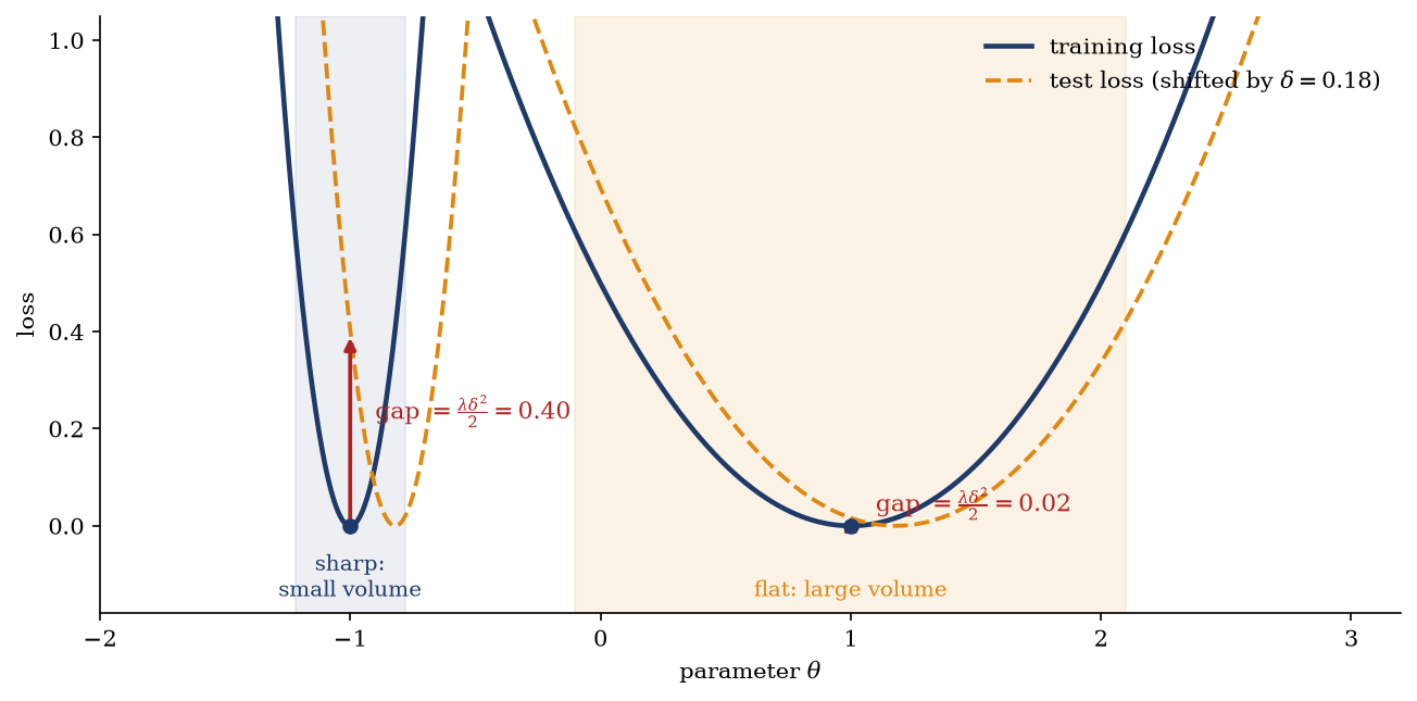
The robustness argument needs one line and no new machinery. Model the passage from training to test as a small displacement of the loss landscape — the test loss is the training loss evaluated on slightly different data, so its minima sit slightly elsewhere. At a training minimum with Hessian \(H\), a shift of effective size \(\delta\) raises the loss by roughly \(\frac{1}{2} \delta^{\mathsf{T}} H \delta\): the generalization gap scales with the curvature. A sharp minimum (\(H\) large) converts a small distribution shift into a large loss increase; a flat one barely notices. Figure 18.1 draws the whole argument: two minima of exactly equal training loss, one narrow and one wide, under a shifted test curve — the sharp minimum’s loss jumps by \(\lambda \delta^2 / 2 = 0.40\), the flat one’s by \(0.02\), a factor of \(\lambda_{\text{sharp}}/\lambda_{\text{flat}} = 25\) with nothing else different between them. (The modern rigorous version of this argument is a PAC-Bayes bound, where flatness controls the generalization gap through a KL term; we keep to the physics telling and name the rigorous one.)
Figure 18.1: The central picture of the lecture: generalization is robustness to the train→test shift. Two minima of the training loss (navy) with exactly equal depth — sharp (\(\lambda = 25\), left) and flat (\(\lambda = 1\), right) — under the test loss (orange dashed), modeled as the same landscape shifted by \(\delta = 0.18\). The gap at each minimum is \(\frac{\lambda \delta^2}{2}\): the sharp minimum jumps by \(0.40\) while the flat one moves by \(0.02\) — a factor \(25\), the curvature ratio, at identical training loss. The shaded bands mark each basin’s width: the volume that the next section converts into an entropy.
The dichotomy is then loss versus free energy. Ranking minima by loss ignores geometry entirely; ranking them by free energy — loss minus temperature times basin entropy — is what a sampler does automatically, and it is the ranking that tracks generalization. Basin entropy is computable through Laplace’s method (Equation 2.2), as the next section shows.
18.3 The engine, part I: flatness is low free energy
The statistical weight of an entire basin, not of its lowest point, is what matters, and Laplace’s method (Equation 2.2) provides it. Consider first the Bayesian question — how much evidence does a basin carry? — at unit temperature. The evidence is the integral of \(e^{-L}\) over the basin (a flat prior over the basin is assumed here; MacKay’s full Occam factor divides this posterior volume by the prior width); expanding \(L\) to second order about the minimum \(\theta^\ast\) and doing the resulting \(d\)-dimensional Gaussian integral,
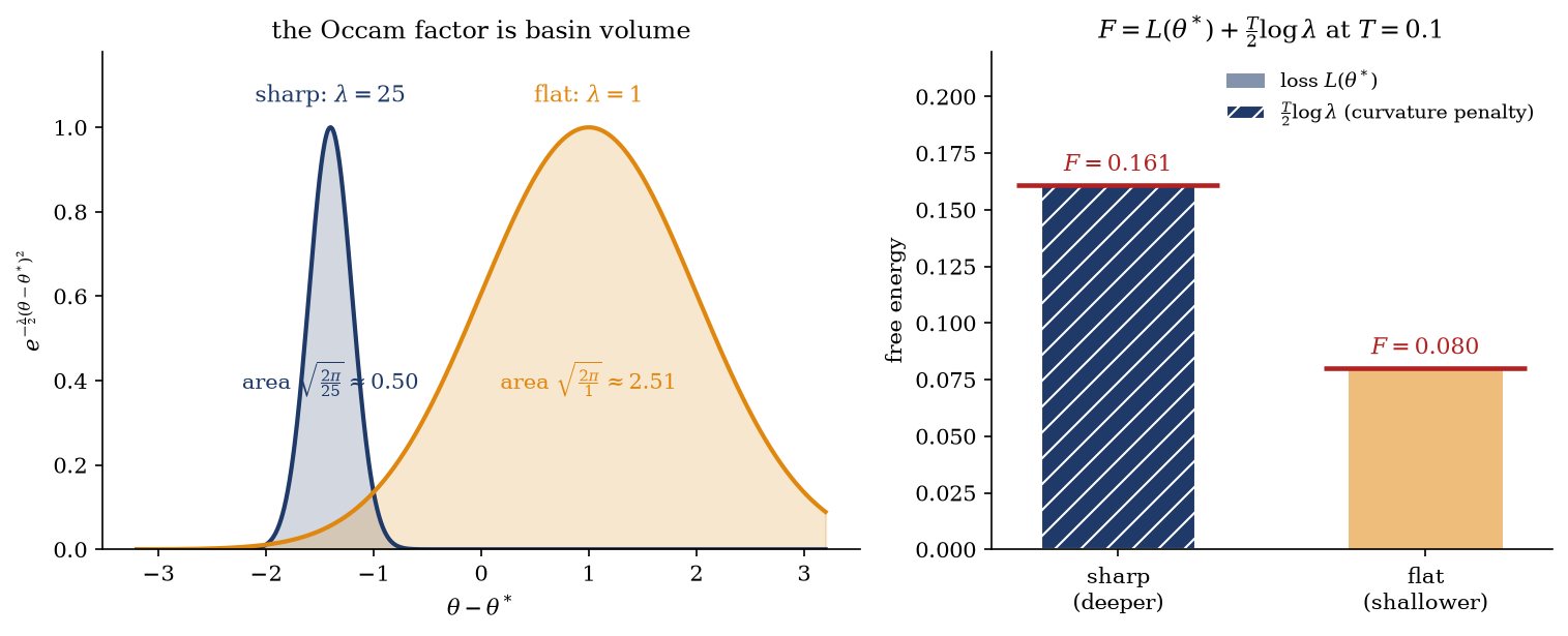
each Hessian eigendirection contributing its one-dimensional width \(\sqrt{2\pi/\lambda_i}\). The prefactor \((2\pi)^{d/2}/\sqrt{\det H}\) is the Occam factor(MacKay 2003): the volume of the basin, large for flat minima and small for sharp ones. Two basins of equal depth do not carry equal evidence — the flat one carries more, in proportion to how many parameter settings inside it fit the data well (Figure 18.2, left). The name is apt: the factor penalizes needlessly precise solutions, exactly Occam’s preference for the less fine-tuned explanation.
The thermodynamic reading follows by attaching the log-volume to the familiar identity. Define the entropy of a basin as the log of its volume, \(S = -\frac{1}{2} \log \det H + \text{const}\); then \(F = \langle E \rangle - TS\) becomes, for a basin explored at temperature \(T\),
\[
\boxed{\;
F \;\approx\; L(\theta^\ast) + \frac{T}{2} \log \det H + \text{const},
\;}
\tag{18.2}\]
free energy of a minimum
the loss at the bottom plus a curvature penalty that grows with temperature. (The same result comes from repeating Equation 18.1 with \(e^{-L/T}\): the basin’s Boltzmann weight is \(e^{-L(\theta^\ast)/T} (2\pi T)^{d/2}/\sqrt{\det H} \equiv e^{-F/T}\), with the \(T\)-dependent constant common to all basins and dropped.) The consequence, drawn in Figure 18.2 (right): a deeper but narrower minimum can have higher free energy than a shallower, wider one. At \(T = 0.1\), a sharp basin with \(\lambda = 25\) and perfect training loss \(L^\ast = 0\) has \(F = 0.161\); a flat basin with \(\lambda = 1\) and worse training loss \(L^\ast = 0.08\) has \(F = 0.080\) — the flat minimum wins on free energy, \(0.080\) against \(0.161\), a margin the loss column cannot see. Whether that ranking governs anything depends on the optimizer actually being a finite-temperature sampler. By the previous lecture’s derivation, it is.
Figure 18.2: Laplace turns basin geometry into statistical weight. Left: the Gaussian factor \(e^{-\frac{\lambda}{2}(\theta - \theta^\ast)^2}\) at a sharp (\(\lambda = 25\)) and a flat (\(\lambda = 1\)) minimum; the enclosed area — the one-dimensional Occam factor \(\sqrt{2\pi/\lambda}\) — is \(0.50\) against \(2.51\): the flat basin holds five times the volume. Right: the free energy Equation 18.2 at \(T = 0.1\) for a sharp-but-deeper minimum (\(L^\ast = 0\), hatched curvature penalty \(\frac{T}{2}\log 25 = 0.161\)) against a flat-but-shallower one (\(L^\ast = 0.08\), penalty zero): the flat minimum has the lower free energy, \(0.080\) against \(0.161\), despite the higher loss.
18.4 The engine, part II: why SGD prefers flat minima
The previous lecture proved that SGD run at fixed \(\eta\) and \(|B|\) samples the Boltzmann distribution \(p_\infty \propto e^{-L/T}\) over parameter space (Equation 17.4). The probability of finding the iterate in a given basin is that distribution integrated over the basin — which is precisely the Laplace computation above:
energy and volume together, with the temperature \(T \propto \eta/|B|\) arbitrating between them. Hot training — small batches, large learning rate — weights volume heavily: the sampler rarely visits narrow wells, however deep, and settles in wide basins. Cold training — large batches — chases depth and finds the sharp minima that Keskar’s experiments caught generalizing poorly (Keskar et al. 2017). The large-batch generalization gap is not a mystery of optimization; it is Equation 18.3 read at low temperature. And the previous lecture’s anisotropy caveat compounds rather than undermines the effect: the gradient noise is anisotropic, largest along the steep directions of the landscape, so SGD is kicked out of sharp wells even faster than a uniform thermostat would manage — a Kramers escape-rate argument we state and do not derive, and exactly the covariance structure the tutorial measures.
Entropy-SGD: the preference as an objective. If flat minima are what we want, we need not rely on SGD’s implicit thermodynamics — optimize for flatness directly. Chaudhari et al. (2017) replace the loss by the local free energy
a log-partition-function over a Gaussian neighborhood of scope\(1/\sqrt{\gamma}\) around \(\theta\) (conventions in the literature differ by harmless prefactors). Small \(F_\gamma\) requires not a low loss at\(\theta\) but a large volume of low loss near\(\theta\): narrow wells contribute almost nothing to the integral and are effectively erased, while wide basins survive. The gradient has a form that makes the objective trainable:
the displacement of \(\theta\) from the mean of the local Gibbs distribution — estimated, in the algorithm, by an inner SGLD chain (Welling and Teh 2011): Week 8’s sampler running as a subroutine inside every outer step, with the scope \(\gamma\) annealed as training proceeds. The free energy entered as a bound (Week 5), became a training loss by amortization (Week 7, Equation 14.6), and now appears as an objective computed by sampling — a partition function estimated with the very MCMC machinery of this module.
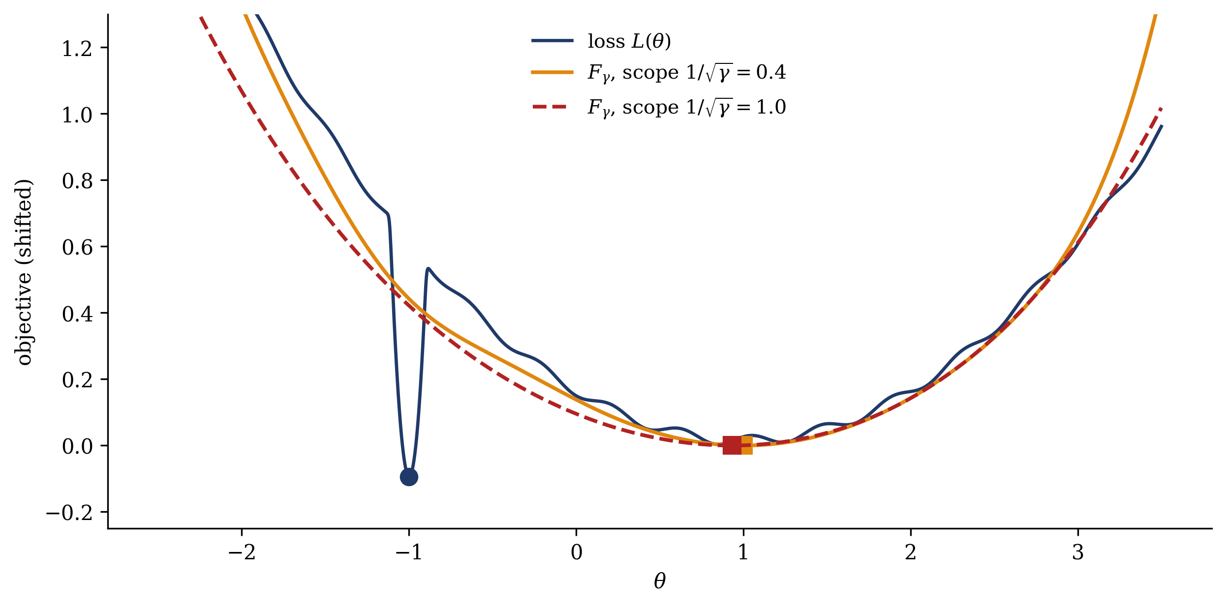
Figure 18.3 shows the objective in action on a landscape designed to test it: a narrow global minimum (lower loss) against a wide valley (higher loss), plus small-scale ruggedness. The smoothed \(F_\gamma\) erases the wiggles and the spike together, and its global minimum relocates to the wide valley — the optimizer that follows \(F_\gamma\) walks past the sharpest, deepest hole in the landscape, by design.
Figure 18.3: The entropy-SGD objective Equation 18.4 on a landscape built to tempt a loss minimizer: the loss \(L(\theta)\) (navy) has its global minimum in a needle at \(\theta = -1\) (depth \(-0.09\), curvature \(\sim 120\)) next to a wide valley at \(\theta = +1\) (minimum \(0\), curvature \(0.3\)), with small wiggles throughout. The local free energy \(F_\gamma\) (each curve shifted so its minimum sits at zero) smooths over a Gaussian neighborhood: at scope \(1/\sqrt{\gamma} = 0.4\) (orange) the wiggles and the needle are erased and the global minimum (square) relocates to the wide valley at \(\theta \approx 1.0\); a wider scope (red dashed) does the same more aggressively. An optimizer descending \(F_\gamma\) walks past the deepest point of the landscape — deliberately.
Take-home 2
Because SGD samples \(e^{-L/T}\), it weights basins by \(e^{-F/T} \sim e^{-L(\theta^\ast)/T}/\sqrt{\det H}\) (Equation 18.3): flat minima are favored, with the strength of the preference set by \(T \propto \eta/|B|\) — large-batch (cold) training finds sharp minima that generalize worse (Keskar et al. 2017), and the anisotropic noise accelerates the escape from sharp wells. Entropy-SGD makes the preference explicit: its objective \(F_\gamma\) (Equation 18.4) is a local free energy whose gradient is computed by an inner SGLD sampler.
18.5 The caveat: flatness is not invariant
The picture above is powerful, and one qualification bounds the claim. Flatness, measured by raw Hessian curvature, is not a property of the function the network computes — it depends on the parameterization. Dinh et al. (2017) make this sharp with a one-line construction: in a ReLU network, scaling one layer’s weights by \(c\) and the next layer’s by \(1/c\) leaves the input–output function — and therefore the test error — exactly unchanged, while rescaling the Hessian’s eigenvalues arbitrarily. Any minimum can be made to look as sharp as desired without touching what the network does; hence the paper’s title, sharp minima can generalize. The free-energy account inherits the same subtlety through its measure: the basin “volume” in Equation 18.1 is a volume in \(\mathrm{d}\theta\), and a reparameterization that reshapes \(\mathrm{d}\theta\) reshapes the entropy with it.
The repair is to measure curvature in a metric the reparameterization cannot fool — the Fisher-information (natural-gradient) geometry, normalized flatness measures, or the PAC-Bayes route, where the generalization bound is stated invariantly from the start; sharpness-aware minimization (SAM, Foret et al. (2021)), the practical descendant of entropy-SGD, minimizes the worst loss in a perturbation ball — though its sharpness too can be fooled by reparameterization until repaired (the scale-invariant ASAM of Kwon et al. 2021). We name these and leave them to the literature. The standing of the lecture’s thesis, then: flat minima generalize is a robust empirical regularity with an illuminating physical mechanism, and it is a leading picture rather than a theorem — the same standing this course gave mean field before its correction (Week 5) and contrastive divergence’s bias (Week 3). Knowing a tool’s domain of validity is part of mastering it.
Trap
Flatness is reparameterization-dependent. Rescaling adjacent ReLU layers by \(c\) and \(1/c\) changes the Hessian arbitrarily without changing the function (Dinh et al. 2017) — raw curvature, and the basin volume behind Equation 18.2, are coordinate quantities. Sharp minima can generalize. The heuristic becomes reliable only in an invariant formulation (Fisher metric, PAC-Bayes, relative sharpness); quote raw \(\det H\) comparisons only between minima of the same parameterization, as done throughout this lecture.
Take-home 3
Raw Hessian flatness can be created or destroyed by reparameterization at fixed network function (Dinh et al. 2017), and the free-energy reading is metric-dependent through the volume measure. The fix is an invariant notion of flatness (Fisher / PAC-Bayes / relative sharpness). Flat-minima-generalize is a powerful leading picture, not a theorem.
18.6 Example: two minima, one temperature dial
We now test the lecture’s claims on a landscape small enough to integrate exactly. Build a one-dimensional loss with a sharp minimum (\(\lambda_s = 25\)) and a flat one (\(\lambda_f = 1\)), and run the two experiments of Figure 18.4.
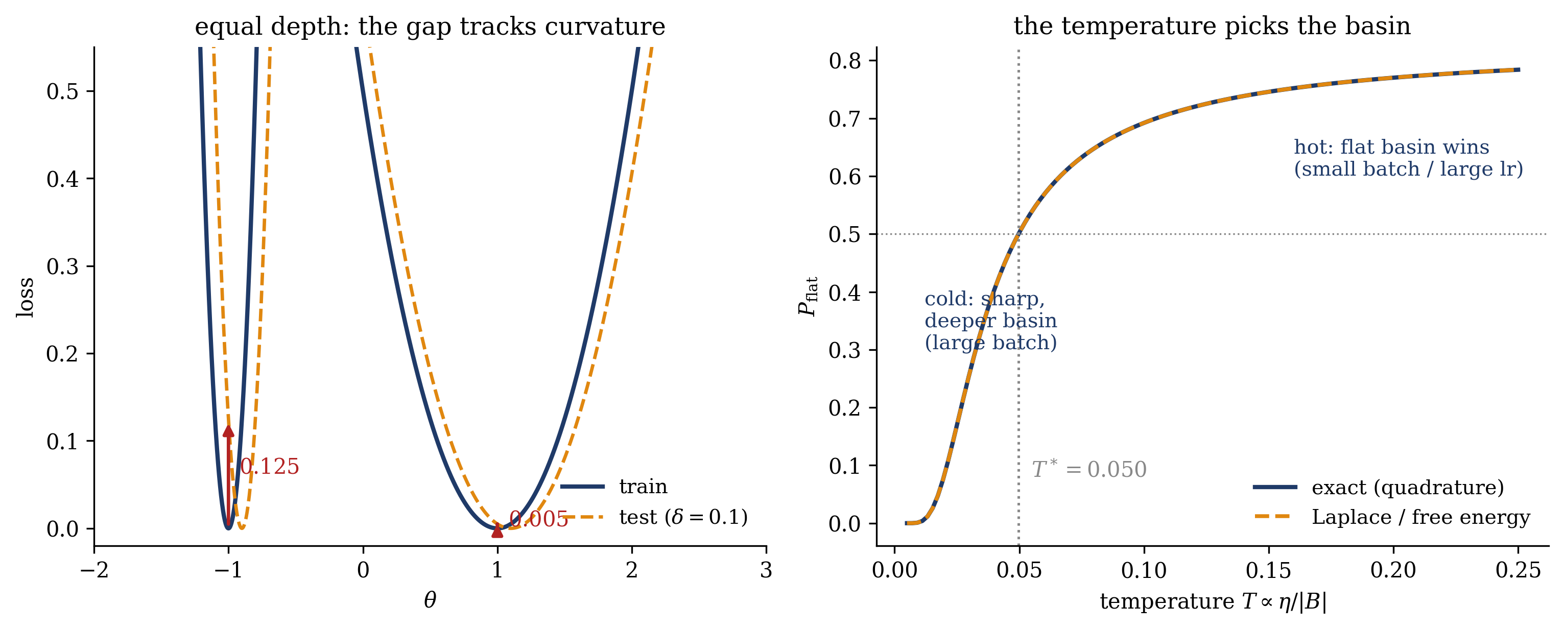
The left panel tests the robustness claim at equal depth: shifting the landscape by \(\delta = 0.1\) raises the loss at the sharp minimum by \(\lambda_s \delta^2/2 = 0.125\) and at the flat one by \(0.005\) — the generalization gap is twenty-five times larger at the sharp minimum, the curvature ratio exactly, with the training losses identical. The right panel then makes the competition unfair: the sharp minimum is made deeper by \(\Delta L = 0.08\), so a zero-temperature loss minimizer would choose it every time. The exact Boltzmann occupation of the flat basin, \(P_{\text{flat}}(T)\), computed by quadrature, tells a different story: cold, the sampler sits in the sharp well (\(P_{\text{flat}} = 0.08\) at \(T = 0.02\)); hot, it lives in the flat one (\(0.77\) at \(T = 0.2\)); and the crossover sits where Equation 18.2 says the two free energies cross,
with the Laplace prediction \(P_{\text{flat}} = [1 + e^{\Delta F / T}]^{-1}\) lying on top of the exact curve across the whole range. Translated through \(T \propto \eta/|B|\), this is Keskar’s experiment in one dimension: batch size and learning rate move the training run along this curve, and which minimum “SGD converged to” is a point on it.
Figure 18.4: The worked example: a double-well loss with a sharp (\(\lambda_s = 25\)) and a flat (\(\lambda_f = 1\)) minimum. Left: at equal depth, the train→test shift \(\delta = 0.1\) opens a gap \(\lambda \delta^2/2\) at each minimum — \(0.125\) (sharp) against \(0.005\) (flat), a factor \(25\) at identical training loss. Right: with the sharp minimum now deeper by \(\Delta L = 0.08\), the equilibrium probability that a sampler of \(e^{-L/T}\) occupies the flat basin, computed exactly by quadrature (navy) and by the Laplace/free-energy formula \(P = [1 + e^{\Delta F/T}]^{-1}\) with \(\Delta F = \Delta L - \frac{T}{2}\log(\lambda_s/\lambda_f)\) (orange dashed, indistinguishable): cold (\(T = 0.02\)) the sampler sits in the sharp-but-deep well (\(P_\mathrm{flat} = 0.08\)); hot (\(T = 0.2\)) in the flat-but-shallow one (\(0.77\)); the crossover \(T^\ast = 2\Delta L / \log(\lambda_s/\lambda_f) \approx 0.050\) (gray dotted) is where the two free energies cross. Through \(T \propto \eta/|B|\), batch size and learning rate select a point on this curve.
18.7 Outlook: Module 3 closes
The tutorial (16–18, Ph12 106) belongs to the previous lecture’s crux — measuring the mini-batch noise covariance against the Fokker–Planck prediction — and today’s lecture has told you what that measurement is for: the anisotropy you will find in \(C(\theta)\) is the mechanism that hurries SGD out of sharp wells and into the flat basins that generalize. You will measure it yourselves — a computation-led week, one machine to a group, opened after the room has predicted what the covariance will look like. The two lectures of the week are one argument: training is Langevin dynamics, and its temperature buys generalization.
Module 3’s arc: Week 8 established that the intractable \(Z\) need not be computed to be used — Metropolis made it cancel (Section 15.3), and annealing turned the sampler into an optimizer by cooling (Chapter 16). Week 9 revealed that the optimizer everyone already runs is such a sampler, with temperature \(\eta/|B|\) (Equation 17.2), equilibrating toward \(e^{-L/T}\) (Equation 17.4). And today that temperature acquired its purpose: it weights basins by free energy (Equation 18.3), preferring the flat, high-entropy minima that survive the train→test shift — with entropy-SGD (Equation 18.4) turning the preference into an explicit objective. Training is sampling; the learning rate is a temperature; generalization is a free energy.
Module 4 takes this machinery to its destination. Week 10 removes the partition function outright — score matching works with \(\nabla_x \log p\), where \(Z\) differentiates to zero (Hyvärinen 2005) — moving the course’s dynamics from parameter space to configuration space at last. Week 11 turns nonequilibrium physics into an estimator: the Jarzynski and Crooks fluctuation theorems (Jarzynski 1997; Crooks 1999) extract free-energy differences from driven, out-of-equilibrium trajectories. And Week 12 runs the previous lecture’s Langevin/Fokker–Planck equations backwards in time to generate: the diffusion model, the course title’s destination. The free energy that has organized every module now builds the samplers of the frontier.
SGD does not chase the lowest loss — it chases the lowest free energy, and a flat minimum is a low-free-energy minimum.
Chaudhari, Pratik, Anna Choromanska, Stefano Soatto, Yann LeCun, Carlo Baldassi, Christian Borgs, Jennifer Chayes, Levent Sagun, and Riccardo Zecchina. 2017. “Entropy-SGD: Biasing Gradient Descent into Wide Valleys.” In International Conference on Learning Representations (ICLR).
Crooks, Gavin E. 1999. “Entropy Production Fluctuation Theorem and the Nonequilibrium Work Relation for Free Energy Differences.”Physical Review E 60 (3): 2721–26. https://doi.org/10.1103/PhysRevE.60.2721.
Dinh, Laurent, Razvan Pascanu, Samy Bengio, and Yoshua Bengio. 2017. “Sharp Minima Can Generalize for Deep Nets.” In Proceedings of the 34th International Conference on Machine Learning (ICML), 70:1019–28. PMLR.
Foret, Pierre, Ariel Kleiner, Hossein Mobahi, and Behnam Neyshabur. 2021. “Sharpness-Aware Minimization for Efficiently Improving Generalization.” In International Conference on Learning Representations (ICLR).
Hinton, Geoffrey E., and Drew van Camp. 1993. “Keeping the Neural Networks Simple by Minimizing the Description Length of the Weights.” In Proceedings of the Sixth Annual Conference on Computational Learning Theory (COLT), 5–13. https://doi.org/10.1145/168304.168306.
Keskar, Nitish Shirish, Dheevatsa Mudigere, Jorge Nocedal, Mikhail Smelyanskiy, and Ping Tak Peter Tang. 2017. “On Large-Batch Training for Deep Learning: Generalization Gap and Sharp Minima.” In International Conference on Learning Representations (ICLR).
MacKay, David J. C. 2003. Information Theory, Inference, and Learning Algorithms. Cambridge: Cambridge University Press.
Welling, Max, and Yee Whye Teh. 2011. “Bayesian Learning via Stochastic Gradient Langevin Dynamics.” In Proceedings of the 28th International Conference on Machine Learning (ICML), 681–88.