26Phase transitions in inference: solvability has a phase diagram
Recommended reading
Core (~1 h).Bahri et al. (2020) §V–VI — the course’s backbone review on the theory side: phase transitions in inference, and the random-matrix and spin-glass pictures of learning that close today’s outlook. Alongside it, the opening two sections of Zdeborová and Krzakala (2016) — the review written from inside the programme this lecture surveys: the easy/hard/impossible picture, message passing as the algorithmic frontier, and the statistical-to-algorithmic gap. This is the one week whose core reading is a pair of reviews rather than a founding paper; the material is a living research programme, not a settled chapter.
Optional background.Decelle et al. (2011) — the detectability threshold derived today, in the original; the flagship inference phase transition. Baik, Ben Arous, and Péché (2005) — the BBP transition, the random-matrix face of the same story. Krzakala et al. (2013) and Saade, Krzakala, and Zdeborová (2014) — the non-backtracking operator and the Bethe–Hessian: how the physics repaired spectral clustering on sparse graphs (today’s numeric uses the latter). Jacot, Gabriel, and Hongler (2018) and Choromanska et al. (2015) — the two outlook pointers, named at the close. Mézard and Montanari (2009) — the textbook home of the whole toolkit.
Prerequisite reminder. From Week 6: belief propagation — the message equation (Equation 12.1), its marginals (Equation 12.2), the Bethe free energy (Equation 12.3), and AMP with its state evolution (Section 12.5). From Week 2: the Hopfield capacity \(\alpha_c \approx 0.138\) (Equation 4.6) and the phase diagram of memory (Figure 4.4). From Week 5: the instability of the disordered state at \(T_c\) (Section 10.2) and Landau’s landscape (Section 10.3). From Week 8: rugged landscapes and metastable traps (Figure 16.1). From the previous lecture: the information bottleneck’s representation transitions in \(\beta\) (Section 25.6). New content: inference problems as disordered systems, the stochastic block model and its detectability threshold, the Kesten–Stigum stability argument, the easy/hard/impossible trichotomy and the statistical-to-algorithmic gap, and the named frontier — neural tangent kernels, random-matrix theory, spin-glass loss landscapes.
26.1 The thread becomes the subject
The course has been saying “phase transition” about learning systems since Week 2, and each time the phrase carried real theorems. Hopfield memory, far from degrading gracefully, shatters at a sharp capacity \(\alpha_c \approx 0.138\) (Equation 4.6), computed by the same replica method that solves spin glasses. The mean-field ferromagnet orders at a sharp \(T_c\) (Section 10.2), and Landau’s expansion (Section 10.3) explained why sharpness is generic. Week 6’s message-passing algorithms converge or fail across sharp boundaries of their own. The previous lecture added a subtler instance: as the trade-off parameter \(\beta\) of the information bottleneck is swept, the optimal representation does not deform smoothly but reorganizes at discrete critical values (Section 25.6). Until today these were features of methods — of memories, approximations, algorithms we built. Today the thread becomes the subject. The problems of inference themselves have phases: tune the signal-to-noise ratio of a statistical-estimation problem and its solvability changes at sharp thresholds, with an order parameter, a symmetry-breaking transition, and — in the most interesting regime — metastability, exactly as in the magnets where this language was invented.
The stance shifts. Modules 1 through 4 used statistical physics to build things: energy-based models, variational approximations, samplers, diffusion processes. This lecture uses it to describe the difficulty of a task — to compute, for a given inference problem, where recovery of a hidden structure is possible at all, and where it is possible efficiently. The object of study is not a new algorithm but the phase diagram of a problem, and the instruments that draw it are precisely the ones this course has already built: belief propagation and its stability (Week 6), the cavity and replica methods (Weeks 2 and 5), approximate message passing and its state evolution (Week 6). This body of work — the statistical physics of inference, associated above all with the programme of Krzakala, Zdeborová, and their collaborators (Zdeborová and Krzakala 2016) — is where the course’s mean-field toolkit is doing frontier research at the time of writing, and it is the last new object of the semester: next week synthesizes and reviews.
The question, then: when does a dataset stop carrying its own explanation — and is the boundary set by information, or by computation?
26.2 Two thresholds, not one
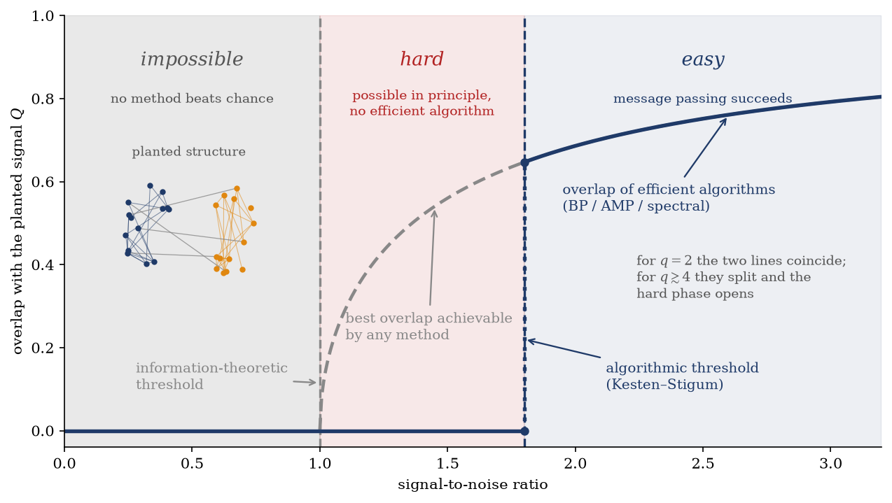
Consider an inference problem with a planted truth — a hidden structure that generated the data — and a signal-to-noise knob. Two different thresholds live on that axis. The information-theoretic threshold is where recovery becomes possible in principle: below it, the posterior simply does not know the answer — no method, however slow, exhaustive, or clever, beats random guessing, because the data are statistically indistinguishable from pure noise. The algorithmic threshold is where some efficient (polynomial-time) method succeeds. The two can coincide, and for the cleanest problem of the day they do. But in general they split, and between them opens a hard phase: a region where the answer is present in the data — an exhaustive search would find it — yet no known efficient algorithm can extract it, and where there is mounting evidence that none exists. Figure 26.1 draws the resulting map, which is today’s central picture.
Figure 26.1: Solvability is a phase diagram. Sweeping the signal-to-noise ratio of a planted inference problem, the overlap between the best reconstruction and the hidden truth (the order parameter) passes through three phases: impossible, where no method beats chance and the achievable overlap is zero; hard, where a positive overlap is achievable in principle (gray dashed) but every known efficient algorithm still returns zero (navy); and easy, where message passing and spectral methods reach the optimum. The two boundaries are the information-theoretic and the algorithmic (Kesten–Stigum) thresholds; for the two-group problem solved in this lecture they coincide, and for \(q \geq 5\) groups (assortative) they separate, opening the hard phase. Inset: the stochastic block model — two planted communities, dense within, sparse between.
The phase boundaries in Figure 26.1 are not metaphors drawn to look thermodynamic; they are computed, and the computation is a free-energy analysis of the posterior. The bridge is one we have crossed repeatedly since Week 3. A posterior distribution over hidden variables is a Boltzmann distribution, \(p(\sigma \mid \text{data}) \propto e^{-E(\sigma)}\) with the negative log-likelihood as energy; the data play the role of quenched disorder, fixed while the hidden variables fluctuate — precisely the structure of the spin glasses of Week 2. Inference questions then are statistical-mechanics questions. Whether the posterior carries any information about the planted truth is the question of whether an order parameter — the overlap between a posterior sample and the truth — is nonzero in the thermodynamic limit; the information-theoretic threshold is a phase boundary of this disordered system, and the algorithmic threshold, as we now derive, is the stability boundary of the dynamics that Week 6 taught us to run on it.
Take-home 1
Inference problems have phases. With a signal-to-noise ratio as control parameter and the overlap with the planted truth as order parameter, recovery switches sharply between impossible and possible — and there are two thresholds, not one: statistically possible, and achievable by an efficient algorithm. When they separate, a hard phase opens between them: the answer is in the data, and no known polynomial-time method can reach it.
26.3 The engine: the detectability threshold
The derivation belongs to the cleanest planted problem in the field: finding two hidden communities in a sparse random graph. The result — a sharp detectability threshold, located by a two-line stability analysis of Week 6’s belief propagation — is due to Decelle et al. (2011), and it is the flagship of the programme.
The model. The stochastic block model (SBM) plants a partition and then hides it in randomness. Take \(n\) nodes and assign each a hidden label \(\sigma_i = \pm 1\), balanced between the two groups. Draw each edge independently: with probability \(a/n\) if the endpoints share a label, \(b/n\) if they differ. The scaling by \(1/n\) keeps the graph sparse — the average degree is \(c = (a+b)/2\), a constant, as in real networks where a person’s friend count does not grow with the population. For \(a > b\) the construction plants assortative communities (Figure 26.1, inset). The inference task: given one graph \(G\) and the parameters, recover the labels better than a coin flip. The natural measure of success is the overlap, \(Q = \tfrac{2}{n}\,\lvert \sum_i \delta_{\hat\sigma_i, \sigma_i} - n/2 \rvert\) in chance-corrected form: \(Q = 0\) is random guessing, \(Q = 1\) is perfect recovery. A single number controls everything below, and we name it now: the reduced signal
\[
\lambda = \frac{a - b}{a + b},
\]
the contrast between in-group and out-group connectivity. (Notation panel, once: \(\lambda\) is a signal-to-noise parameter throughout this section, not an eigenvalue — although in the spiked-matrix section below the signal strength will be an eigenvalue, which is no coincidence. The letter \(c\) is the average degree, not a capacity; Week 2’s \(\alpha\) is retired.)
The posterior is a Boltzmann distribution. Bayes with a flat prior gives \(p(\sigma \mid G) \propto P(G \mid \sigma)\), and the likelihood factorizes over pairs — present edges and absent ones both count as evidence:
Take the log and use \(\sigma_i \sigma_j = \pm 1\) to write each factor in Ising form. For an edge, \(\ln c_{\sigma_i\sigma_j} = \tfrac{1}{2}\ln(ab) + \tfrac{1}{2}\ln(a/b)\, \sigma_i \sigma_j\): a coupling. For a non-edge, \(\ln(1 - c_{\sigma_i\sigma_j}/n) = -c_{\sigma_i\sigma_j}/n + \mathcal{O}(n^{-2})\), which contributes \(-\tfrac{a-b}{2n}\,\sigma_i\sigma_j\) per pair: a coupling as well, weak but acting between all pairs. Collecting constants into the normalization,
the SBM posterior: a dilute ferromagnet with a balance constraint
Read the two terms as a physicist. The first is an Ising ferromagnet (\(a > b\) makes \(J > 0\)) living on the observed graph — the data are the lattice, which is the quenched disorder of this problem. The second is an infinitesimal all-to-all antiferromagnet; summed over \(n\) neighbors it acts as a self-consistent field \(-\tfrac{a-b}{2}\, \bar m\) opposing the mean magnetization \(\bar m\), and its job is bookkeeping: it encodes the knowledge that the groups are balanced, so the posterior must not simply magnetize. Sampling this Boltzmann distribution at temperature \(1\)is Bayesian inference on the SBM. The community structure we seek is a hidden ordering of a dilute magnet, and “can the communities be found?” becomes “does this magnet order along the planted direction?”
The Nishimori simplification. One structural fact makes the analysis tractable. We are inferring with the same model that generated the data — the true \(a\), \(b\) enter the posterior coupling \(J\). This Bayes-optimal setting places the system on its Nishimori line, where identities special to the planted ensemble hold: the planted configuration is statistically indistinguishable from a typical posterior sample, and the overlap between two independent posterior samples equals, on average, the overlap of either with the truth. Critically, on this line the equilibrium free energy is exactly replica-symmetric — the static glass transitions that haunt Week 2’s memory at overload cannot occur at Bayes optimality (Zdeborová and Krzakala 2016). That is why the thresholds below are sharp and computable: the replica-symmetric cavity analysis — belief propagation, by Week 6’s dictionary — is asymptotically exact here. Metastable states are demoted rather than excluded: they may still trap dynamics, and that loophole is exactly where the hard phase will come from.
Belief propagation and the fixed point of ignorance.Equation 26.1 is a pairwise Ising model, so Week 6’s machinery applies verbatim: messages \(u_{k \to i}\) on the directed edges of \(G\), the message equation Equation 12.1 with \(\beta = 1\) and uniform coupling \(J\), cavity fields \(h_{i \to j} = \sum_{k \in \partial i \setminus j} u_{k \to i}\), and the weak all-pairs term treated at the level of Week 5’s naive mean field — a single global field that pins the total magnetization to zero and otherwise sits out the argument. The sparse graph is locally tree-like — the neighborhood of a typical node contains no loop out to distance \(\mathcal{O}(\ln n)\) — so BP is asymptotically exact here, as promised in Week 6 and guaranteed by the Nishimori property.
Whatever the parameters, this BP always admits one particular fixed point: all messages zero, \(u_{k \to i} = 0\) on every directed edge — by Equation 12.1, \(\tanh(0) = 0\) propagates to itself. At this fixed point every marginal is \(1/2\) and the algorithm asserts total ignorance: every node is equally likely in either group. This solution must exist because the model Equation 26.1 is exactly symmetric under a global flip of all labels, so the uninformative state is protected by symmetry at every signal strength, however strong the planted structure. Detection therefore cannot be a question of whether an informative solution appears; it is a question of whether the state of ignorance is stable. If a small perturbation of the messages dies out under iteration, BP relaxes back to knowing nothing. If it grows, the symmetric state collapses and the messages flow toward an informative fixed point correlated with the planted labels. We have met this logic twice: it is the instability of \(m = 0\) at the Curie point (Section 10.2), and the birth of Landau’s ordered minima (Section 10.3), replayed on an inference problem.
Linearize. Perturb around ignorance: small cavity fields \(h_{k \to i} = \varepsilon_{k \to i}\). Week 6’s message equation linearizes in one step,
The reduced signal is the bond attenuation. Week 6 read the message equation as “a weak bond whispers”; here every bond whispers with the same factor \(\lambda\), and the linearized recursion for the cavity fields is simply
Count. Each iteration multiplies a perturbation by \(\lambda\) and branches it through the graph. On the locally tree-like SBM the number of neighbors feeding a message — the excess degree — is Poisson with mean \(c\), so after \(d\) generations a disturbance at the root has descended a tree with \(c^d\) leaves, each reached along a path of attenuation \(\lambda^d\). Whether the disturbance survives depends on how the leaf contributions combine, and here sits the one subtle step of the derivation. ① A coherent perturbation — all leaves nudged toward \(+\) — would return to the root amplified by \((c\lambda)^d\). But that mode is the global magnetization, which the balance field of Equation 26.1 holds at zero, and ordering “everyone in group \(+\)” carries no information about the partition anyway. ② The perturbations that matter are the incoherent ones the random graph itself seeds: independent, random-signed nudges of the leaves, mean zero. Their sum at the root has zero mean, and the information rides on its variance — \(c^d\) independent contributions, each of size \(\lambda^d\):
The uninformative fixed point is unstable — a whisper of community structure is amplified rather than forgotten — precisely when \(c\lambda^2 > 1\), the Kesten–Stigum condition, first found in the theory of multitype branching processes (Kesten and Stigum 1966), later identified as the reconstruction threshold for broadcasts on trees, and rediscovered here as the stability boundary of an algorithm. Substituting \(\lambda = (a-b)/(a+b)\) and \(c = (a+b)/2\) turns the condition into the parameters of the model:
\[
\boxed{\;
(a - b)^2 = 2\,(a + b)
\quad\Longleftrightarrow\quad
c\,\lambda^2 = 1
\;}
\tag{26.4}\]
the detectability threshold (Decelle et al. 2011)
Above this line a positive overlap with the planted labels is achievable, and belief propagation achieves it in linear time; below it, for two balanced groups, the physics analysis of Decelle et al. (2011) concluded that the sparse SBM is information-theoretically indistinguishable from an Erdős–Rényi graph of the same density — the communities are present in the generator and absent from the data — a conjecture since proved rigorously, completing one of the programme’s cleanest exchanges between physics and mathematics (Zdeborová and Krzakala 2016). The detectability threshold is thus the point where the posterior’s symmetric state loses stability — a symmetry-breaking phase transition, the mathematics of a magnet ordering, evaluated on an inference problem, with Week 6’s algorithm as the order-parameter dynamics.
The numbers show how sharp the line is. At average degree \(c = 3\), the threshold sits at \(\lambda = 1/\sqrt{3} \approx 0.577\), i.e. \(a \approx 4.73\), \(b \approx 1.27\). Now plant communities with \(a = 4.5\) and \(b = 1.5\): every node has three times more neighbors inside its group than outside, a contrast that would be unmistakable in any drawing of the model — and yet \(c\lambda^2 = 0.75 < 1\), so no method, spectral, message-passing, or exhaustive, recovers anything. A three-to-one contrast is completely invisible below the line. That is what “the data stop carrying their own explanation” means quantitatively, and Section 26.6 measures it.
Take-home 2
Two planted communities in a sparse graph are detectable if and only if \((a-b)^2 > 2(a+b)\) (Equation 26.4) — the point where the uninformative fixed point of Week 6’s belief propagation goes linearly unstable, with growth factor \(c\lambda^2\) (Equation 26.3). Solvability is a symmetry-breaking phase transition in the posterior, and the mean-field toolkit of Module 2 is the instrument that locates it.
26.4 Easy, hard, impossible
For two balanced groups the story ends cleanly: the Kesten–Stigum line is both thresholds at once — where efficient detection begins and where any detection begins — and the phase diagram has just two regions, easy and impossible. The general picture is richer, and the enrichment is the field’s central discovery. Increase the number of groups \(q\), and the two thresholds separate: for \(q \geq 5\) in the symmetric assortative model (\(q \geq 4\) in the disassortative / planted-colouring case, and earlier still with unbalanced groups or broad degree distributions), the information-theoretic threshold slides below the Kesten–Stigum line (Decelle et al. 2011; Zdeborová and Krzakala 2016). In the window between them, a typical instance contains enough information to recover the communities — the posterior, exhaustively explored, knows the answer — but belief propagation, AMP, spectral methods, and every other known polynomial-time algorithm return noise. This is the hard phase of Figure 26.1, and the statistical-to-algorithmic gap between the two lines is the object the field now studies most intently, because it appears to be a law about computation itself, discovered with the tools of statistical mechanics.
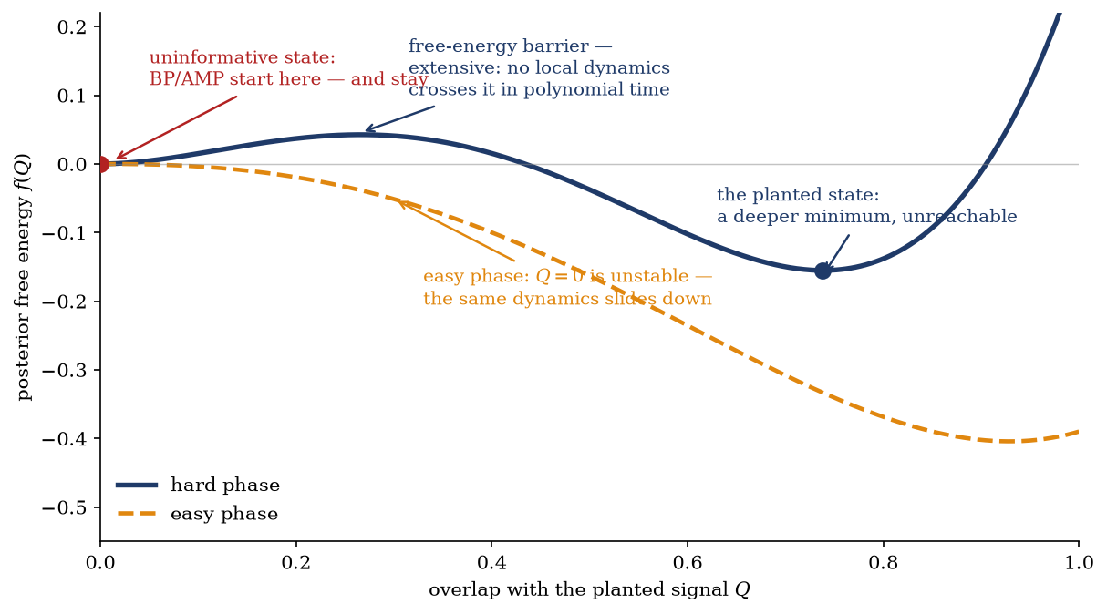
Figure 26.2: Why “hard” is a physics statement. In the hard phase (navy) the posterior free energy over the overlap coordinate has two minima: the uninformative state at \(Q = 0\), locally stable, where message passing and every local dynamics begin — and where they stay, because the barrier between the minima is extensive and cannot be crossed in polynomial time. The informative state exists and is thermodynamically favored; it is simply unreachable. In the easy phase (orange, dashed) the barrier is gone, \(Q = 0\) is unstable (Equation 26.3), and the same dynamics slides down to the answer. The hard phase is Week 8’s metastability, relocated from configuration space to the space of inference states.
Why should a possible problem be hard? The physics answer is drawn in Figure 26.2, and it reuses a landscape the course has already built. Compute the Bethe free energy (Equation 12.3) of the posterior as a function of the overlap \(Q\). In the hard phase it has two local minima: the uninformative state at \(Q = 0\), still locally stable since \(c\lambda^2 < 1\), and an informative state at \(Q > 0\), now lower in free energy — the global minimum, which is why exhaustive search succeeds and the information-theoretic threshold has passed. Between them stands an extensive free-energy barrier. Every algorithm we possess for such models is local — BP and AMP iterate small updates, MCMC flips spins, gradient methods take small steps — and a local dynamics started at (or near) ignorance equilibrates into the metastable minimum and stays: the escape time is exponential in \(n\), Week 8’s quench-into-a-glass (Figure 16.1) with the annealing schedule powerless because the barrier does not soften. The transition at the information-theoretic threshold is first-order in the Landau sense (Section 10.3): the informative minimum appears at finite \(Q\) and crosses below the uninformative one while both remain locally stable, and algorithmic hardness lives exactly in the coexistence window. Hardness, in this picture, is metastability — a statement about the geometry of the posterior, not about any particular algorithm’s cleverness, which is why the conjecture that no polynomial algorithm beats Kesten–Stigum here has survived a decade of attempts and now anchors average-case complexity theory well outside physics (Zdeborová and Krzakala 2016).
26.5 One transition, many problems
The SBM would be a curiosity if its phase diagram were its own. It is not; the same trichotomy, computed by the same methods, organizes the canonical estimation problems of high-dimensional statistics. We state the two landmark cases result-first — each is a lecture in the source material, and the point here is the pattern.
Spiked matrices and the BBP transition. Plant a rank-one signal in symmetric noise: observe \(Y = \lambda\, v v^{\mathsf T} + W\) with \(v\) a hidden unit vector, \(\lambda\) the signal strength, and \(W\) a Wigner matrix whose spectrum fills the semicircle on \([-2, 2]\). (As promised, the signal strength of this paragraph is an eigenvalue.) This is low-rank matrix estimation stripped to its core — the planted ancestor of PCA, factor analysis, and the low-rank decompositions of recommender systems. The spectrum of \(Y\) undergoes a sharp transition, first located by Baik, Ben Arous, and Péché (2005) in the sample-covariance setting and carrying their initials (BBP): for \(\lambda \leq 1\) the signal is swallowed by the bulk and the top eigenvector is asymptotically orthogonal to \(v\) — PCA returns pure noise; for \(\lambda > 1\) an outlier eigenvalue detaches from the bulk edge at \(\lambda + 1/\lambda\) and the leading eigenvector locks onto the signal with squared overlap \(1 - \lambda^{-2}\). A rank-one perturbation of vanishing relative norm either vanishes entirely from the spectrum or reorganizes it, with nothing in between. For the symmetric \(\pm 1\) signal the three lines — spectral, message-passing, information-theoretic — coincide at \(\lambda = 1\); make the signal sparse, and they separate, opening the same hard phase as the many-group SBM, this time in sparse PCA (Zdeborová and Krzakala 2016). AMP (Section 12.5), whose state evolution tracks its own accuracy exactly, is the instrument that draws these Bayes-optimal curves.
Planted clique, the starkest gap. Hide a clique of size \(k\) in a uniformly random graph on \(n\) nodes. Information-theoretically the clique is detectable once \(k \gtrsim 2\log_2 n\), since that is where it begins to exceed the largest clique the noise produces by chance. Every known polynomial-time algorithm, spectral or message-passing or otherwise, needs \(k\) of order \(\sqrt{n}\). Between a logarithmic and a polynomial clique size stretches the widest hard phase known — not a sliver between nearby thresholds but essentially the entire parameter range — which has made planted clique the drosophila of average-case hardness: a problem now used as a primitive, with the hardness of other tasks established by reduction to it.
The physics also repairs the algorithms. The programme’s traffic is not one-way from problems to phase diagrams; the free-energy picture has produced better algorithms. Naive spectral clustering — take the second eigenvector of the adjacency matrix, threshold its signs — fails well above the detectability threshold on sparse graphs, for a concrete reason: with Poisson degrees the largest degree grows like \(\ln n / \ln\ln n\), and the top adjacency eigenvectors localize on these hubs (Week 4 met the same pathology in another guise), drowning the community mode. The repair came from the cavity method: the non-backtracking operator — the linearization of BP, Equation 26.2, read as a matrix on directed edges, forbidden from immediately retracing its last step — has a clean spectrum whose informative eigenvalues detach exactly at Kesten–Stigum (Krzakala et al. 2013). Its symmetric, \(n \times n\) stand-in is the Bethe–Hessian\(H(r) = (r^2 - 1)\mathbb{1} - rA + D\) with \(r = \sqrt{c}\) (here \(A\) is the adjacency matrix, \(D\) the diagonal degree matrix): literally the Hessian of Week 6’s Bethe free energy (Equation 12.3) at the uninformative point, whose negative directions are the unstable community modes (Saade, Krzakala, and Zdeborová 2014). The result is a spectral algorithm that works down to the theoretical limit, obtained by differentiating a free energy twice; the numeric below runs it.
26.6 Example: the threshold, measured
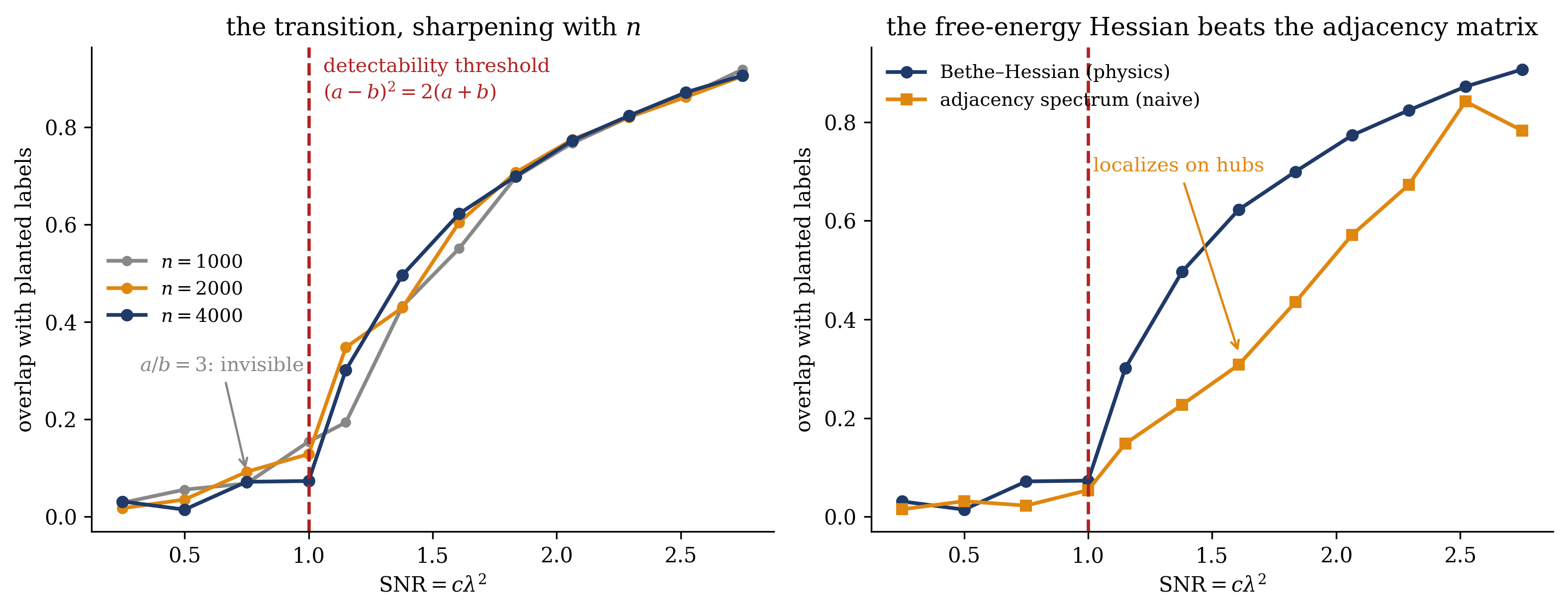
The boxed line Equation 26.4 makes a falsifiable claim: plant communities below it and every method returns noise; cross it and a linear-time algorithm finds them. The experiment generates symmetric two-group SBMs at fixed average degree \(c = 3\), sweeps the signal-to-noise ratio \(\mathrm{SNR} = c\lambda^2 = (a-b)^2/[2(a+b)]\) through \(1\), recovers labels with the Bethe–Hessian, and measures the chance-corrected overlap — including, at \(\mathrm{SNR} = 0.75\), the three-to-one graphs the engine section promised were invisible.
Figure 26.3: The detectability threshold, measured (symmetric two-group SBM, average degree \(c = 3\), four graphs per point). Left: chance-corrected overlap between recovered and planted labels for the Bethe–Hessian spectral method (Saade, Krzakala, and Zdeborová 2014), against the signal-to-noise ratio \(\mathrm{SNR} = c\lambda^2 = (a-b)^2/[2(a+b)]\). Below the threshold \(\mathrm{SNR} = 1\) of Equation 26.4 (red line) the overlap sits at the noise floor — at most \(0.07\) for \(n = 4000\), including the \(a/b = 3\) graphs at \(\mathrm{SNR} = 0.75\) — and above it the overlap rises continuously from zero. The residual overlap at the threshold itself shrinks with system size (\(0.16 \to 0.07\) from \(n = 1000\) to \(4000\)): the transition is sharp only as \(n \to \infty\), like every phase transition of the course. Right: the physics-derived operator against naive adjacency clustering at \(n = 4000\) — near \(\mathrm{SNR} \approx 1.8\) the Bethe–Hessian reaches an overlap of \(0.70\) while the adjacency eigenvector, partially localized on high-degree nodes, delivers \(0.44\); the naive spectrum needs roughly half again as much signal for the same accuracy.
Figure 26.3 confirms the threshold quantitatively. Left panel: below the red line the overlap is indistinguishable from noise at every size — the \(a/b = 3\) graphs sit at \(0.07\) — and the rise beyond it steepens as \(n\) grows, the familiar finite-size rounding of a genuine transition (compare the Hopfield fold of Week 2 and the Ising peak of Week 1’s tutorial). Below the line there is no algorithmic parameter left to tune; the information is gone from the data, not hidden from the method. Right panel: the gap between the navy and orange curves is the practical gain of Section 26.5 — two eigenvector computations of identical cost, one guided by the Bethe free energy and one not, separated by a factor of \(1.6\) in overlap through the transition region.
Trap
Four ways to misquote a detectability threshold. ① Detection is not exact recovery.Equation 26.4 is the line for beating chance — a positive overlap. Recovering every label correctly is a different, stricter threshold, living in a denser regime (average degree growing like \(\ln n\)); quoting the constant-degree formula for it is a category error. ② “Impossible” and “no efficient algorithm” are different lines. The information-theoretic and algorithmic thresholds coincide for two balanced groups only; conflating them in general erases the hard phase, which is the field’s central object. ③ The uninformative fixed point always exists — detectability is about its stability, not its presence. The symmetric solution is protected by the label-flip symmetry at every SNR; nothing “appears” at the threshold except an instability, cf. Equation 26.3. ④ The threshold statement is a sparse-regime statement.\((a-b)^2 = 2(a+b)\) is derived at constant average degree \(c\); in dense scalings the constants and even the questions change. State the regime before quoting the line.
Take-home 3
On sparse two-group SBMs the measured overlap sits at the noise floor below \((a-b)^2 = 2(a+b)\) and rises continuously above it, sharpening with system size — a phase transition observed in an inference problem. The same physics that predicts the line also builds the better algorithm: the Bethe–Hessian (the curvature of Week 6’s Bethe free energy at the point of ignorance) detects down to the threshold where the naive adjacency spectrum, localized on hubs, fails. In the multi-group and sparse-signal versions the statistical and algorithmic lines separate, and the gap between them is the frontier.
Inference has phases: below a sharp signal threshold the data hide a structure that no efficient algorithm — and sometimes no method at all — can recover; statistical physics draws that line and characterizes the region between the possible and the efficient.
26.7 Outlook: where the physics is going
The detectability threshold is one exhibit from an active research programme, and this section names three neighbors without deriving them, following Bahri et al. (2020) §V–VI. The neural tangent kernel(Jacot, Gabriel, and Hongler 2018) is the infinite-width limit in which a deep network’s training linearizes: the network trains as a kernel machine with a kernel fixed at initialization, generalization becomes computable — and the limit simultaneously proves that in this lazy regime no features are learned at all, which converts “how do networks learn features?” from a slogan into a sharply posed open problem about finite-width corrections. Random-matrix theory — the BBP transition’s home discipline — now computes learning curves for high-dimensional regression and classification, including the double-descent phenomenon in which test error peaks at the interpolation threshold and falls again beyond it: generalization behavior organized, once more, by the spectrum of a random matrix. And the loss landscapes of deep networks have a spin-glass description: under simplifying assumptions, Choromanska et al. (2015) mapped deep-network losses to the Sherrington–Kirkpatrick-family models of Week 2, with exponentially many critical points stratified by index and the low-loss minima concentrated in a narrow band — a picture whose assumptions are unrealistic and whose qualitative predictions have nonetheless kept matching experiments, in the same spirit as Week 9’s flat-minima story. Each of these is the same intellectual move this lecture made on the SBM: take a question about learning, identify the disordered system it secretly is, and compute.
The tutorial (16–18, Ph12 106) belongs to the previous lecture, not this one: the information-bottleneck objective derived as constrained free-energy minimization, and the IB curve computed for a small classifier, starting from the previous lecture’s Lagrangian (Equation 25.1) rather than today’s threshold. The IB’s representation transitions in \(\beta\) are, in hindsight, the first inference phase transition of the week. And with today, the course’s new material ends. Next week’s Lecture 1 is the synthesis: the whole semester read as one free-energy calculation, from Hopfield’s magnet to the diffusion model’s reverse SDE to today’s phase diagram of solvability. Next week’s Lecture 2 is the exam review. Statistical physics entered machine learning as a supplier of models and methods, but its deepest current contribution runs the other way — it is becoming the theory of what learning problems are, and the phase diagram of inference is its first map.
Bahri, Yasaman, Jonathan Kadmon, Jeffrey Pennington, Sam S. Schoenholz, Jascha Sohl-Dickstein, and Surya Ganguli. 2020. “Statistical Mechanics of Deep Learning.”Annual Review of Condensed Matter Physics 11: 501–28. https://doi.org/10.1146/annurev-conmatphys-031119-050745.
Baik, Jinho, Gérard Ben Arous, and Sandrine Péché. 2005. “Phase Transition of the Largest Eigenvalue for Nonnull Complex Sample Covariance Matrices.”Annals of Probability 33 (5): 1643–97. https://doi.org/10.1214/009117905000000233.
Choromanska, Anna, Mikael Henaff, Michael Mathieu, Gérard Ben Arous, and Yann LeCun. 2015. “The Loss Surfaces of Multilayer Networks.” In AISTATS 2015, PMLR, 38:192–204.
Decelle, Aurélien, Florent Krzakala, Cristopher Moore, and Lenka Zdeborová. 2011. “Asymptotic Analysis of the Stochastic Block Model for Modular Networks and Its Algorithmic Applications.”Physical Review E 84 (6). https://doi.org/10.1103/PhysRevE.84.066106.
Jacot, Arthur, Franck Gabriel, and Clément Hongler. 2018. “Neural Tangent Kernel: Convergence and Generalization in Neural Networks.” In NeurIPS. Vol. 31.
Kesten, Harry, and Bernt P. Stigum. 1966. “Additional Limit Theorems for Indecomposable Multidimensional Galton-Watson Processes.”Annals of Mathematical Statistics 37 (6): 1463–81. https://doi.org/10.1214/aoms/1177699139.
Krzakala, Florent, Cristopher Moore, Elchanan Mossel, Joe Neeman, Allan Sly, Lenka Zdeborová, and Pan Zhang. 2013. “Spectral Redemption in Clustering Sparse Networks.”Proceedings of the National Academy of Sciences 110 (52): 20935–40. https://doi.org/10.1073/pnas.1312486110.
Mézard, Marc, and Andrea Montanari. 2009. Information, Physics, and Computation. Oxford: Oxford University Press.
Saade, Alaa, Florent Krzakala, and Lenka Zdeborová. 2014. “Spectral Clustering of Graphs with the Bethe Hessian.” In NeurIPS, 27:406–14.
Zdeborová, Lenka, and Florent Krzakala. 2016. “Statistical Physics of Inference: Thresholds and Algorithms.”Advances in Physics 65 (5): 453–552. https://doi.org/10.1080/00018732.2016.1211393.