17 SGD as Langevin dynamics: the temperature of training

17.1 Training is sampling

Week 8 ended on a bridge built deliberately: SGLD adds Gaussian noise to a gradient step and thereby samples \(e^{-L/T}\) at a temperature set by that injected noise (Welling and Teh 2011) — while the same lecture’s closing scaling argument already hinted that plain SGD carries a temperature set by the step size itself. But SGLD injects its noise explicitly, and the bridge appeared to depend on that injection. It does not. Ordinary stochastic gradient descent — the algorithm training every network in this course, with no noise added by anyone — is already a noisy dynamics, because each step evaluates the gradient on a random mini-batch rather than the full dataset. A mini-batch gradient is the true gradient plus a zero-mean fluctuation, and a particle descending a potential under zero-mean kicks performs Brownian motion in a potential, not optimization as the textbooks draw it — the problem Langevin (1908) wrote the equation for.

That reframe is the lecture’s central idea, and it has a long history. In 1908 Langevin described a Brownian particle by Newton’s equation plus two new forces, a friction and a random thermal kick, and showed the pair reproduces Einstein’s diffusion. Fokker (1914) and Planck (1917) then wrote the complementary equation: not for the particle’s trajectory but for the evolution of its probability distribution, whose long-time limit is the Boltzmann distribution. A century later, Mandt, Hoffman, and Blei (2017) observed that the SGD iterate satisfies Langevin’s equation with the loss as the potential and the mini-batch fluctuations as the thermal kicks — so the Fokker–Planck equation governs the distribution of the parameters during training, and its stationary solution answers the question what distribution does training converge to?

The stationary distribution turns out to be a Boltzmann distribution over the loss, \(p_\infty \propto e^{-L/T}\), at a temperature \(T \propto \eta/|B|\) — the learning rate over the batch size. The Boltzmann law of Week 1 returns a final time in this module, now with the parameters \(\theta\) as the configuration and the loss \(L\) as the energy. Training is sampling; SGD thermalizes around a minimum rather than coming to rest at it; and the two most-tuned hyperparameters in deep learning are two dials on a single physical quantity. The derivation occupies the two engine sections; the consequences and caveats follow, and the tutorial measures the resulting prediction.

Take-home 1

SGD is not deterministic descent: the random mini-batch makes its gradient noisy, and noisy descent in a potential is Langevin (Brownian) dynamics — \(\theta\) a particle, the loss a potential, the mini-batch fluctuations thermal kicks. SGD fluctuates around minima rather than resting at them. Training is sampling, and the learning rate sets the temperature.

17.2 Optimizer or sampler

The same algorithm admits two readings. Read as an optimizer, SGD’s noise is a nuisance: it prevents convergence to the minimizer, and the practitioner anneals it away. Read as a sampler, the noise is the mechanism: SGD draws from a distribution concentrated on low loss, the noise strength decides how concentrated, and “convergence” means the distribution has stopped changing, not the iterate. Both readings are correct; the sampler reading is the one with predictive power, because it attaches a number — a temperature — to the vague notion of “how much SGD explores.”

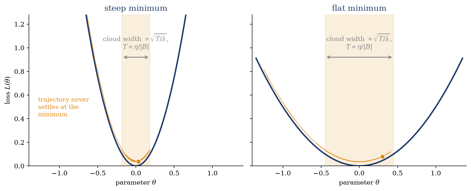
Figure 17.1 draws the sampler reading before any equation. The iterate descends into a well of the loss and then does not stop: it jitters, indefinitely, in a stationary cloud around the minimum. The cloud’s width will come out as \(\sqrt{T/\lambda}\) — temperature over local curvature — so the same temperature makes a narrow cloud in a steep minimum and a wide one in a flat minimum. Both knobs of practice collapse into that single \(T\): raising the learning rate \(\eta\) heats the dynamics, and enlarging the batch \(|B|\) — averaging away more of the gradient noise — cools it. The whole phenomenology of “large batches converge sharply, small batches explore” is one statement about one number.

Figure 17.1: The central picture of the lecture: SGD as a Brownian particle in the loss landscape. In both panels the iterate (orange trajectory) falls into the well and then never settles — it thermalizes into a stationary cloud (shaded band) around the minimum, of width \(\propto \sqrt{T/\lambda}\) for local curvature \(\lambda\), with the temperature \(T \propto \eta/|B|\) set by the learning rate over the batch size. Left: a steep minimum confines the cloud tightly. Right: at the same temperature, a flat minimum leaves a wide cloud — the geometry that becomes the flat-minima story of the next lecture.

A distinction about spaces is essential here, because the course’s spine depends on it. Today’s dynamics runs in parameter space: the variable is \(\theta\), the gradients are \(\nabla_\theta\), and the energy is the loss — the same space where Week 3 met its training obstruction \(\nabla_\theta \log Z\) (Equation 5.5). It is not the configuration-space dynamics over data \(x\) that Week 10 will need for score matching, where the object is \(\nabla_x\) and the partition function conveniently drops out. Same machinery, two different spaces; we will run it in the other space soon enough. Two notational points: \(W\) below is the Wiener process, not a weight matrix; and \(T\) is a derived property of the algorithm, not an external thermostat — nobody set it, but it is there.

17.3 The engine, part I: the noise in the gradient

The empirical loss is an average over the dataset, \(L(\theta) = \frac{1}{N} \sum_{i=1}^N \ell_i(\theta)\), and a full gradient costs \(N\) per-sample gradients. SGD instead draws a random mini-batch \(B \subset \{1, \dots, N\}\) and uses

\[ \nabla \hat{L}_B(\theta) \;=\; \frac{1}{|B|} \sum_{i \in B} \nabla \ell_i(\theta), \]

an average of \(|B|\) randomly selected per-sample gradients. Averages of many random terms are Week 1’s home ground: this estimator is unbiased, \(\langle \nabla \hat{L}_B \rangle = \nabla L\), and its fluctuations shrink as \(1/|B|\) in covariance. Writing \(C(\theta) = \frac{1}{N} \sum_i \big(\nabla \ell_i - \nabla L\big)\big(\nabla \ell_i - \nabla L\big)^{\mathsf{T}}\) for the covariance of the per-sample gradients — the dataset’s intrinsic gradient spread at \(\theta\) —

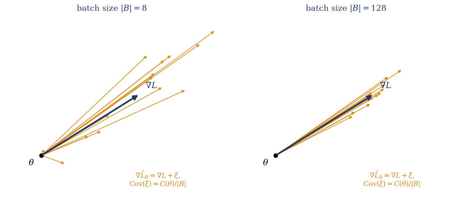
\[ \nabla \hat{L}_B \;=\; \nabla L + \xi, \qquad \langle \xi \rangle = 0, \qquad \mathrm{Cov}(\xi) \;=\; \frac{C(\theta)}{|B|}, \tag{17.1}\]

mini-batch gradient noise

and for \(|B|\) reasonably large the central limit theorem makes \(\xi\) Gaussian. (For sampling without replacement a finite-population factor \(1 - |B|/N\) multiplies the covariance; for the usual \(|B| \ll N\) it is invisible and we drop it.) Figure 17.2 shows what Equation 17.1 looks like: a scatter of mini-batch gradients around the true one, tightening as the batch grows — and, in general, spread unequally across directions, a detail that returns in Section 17.5 with consequences.

Figure 17.2: The engine’s first picture: the mini-batch gradient is the full gradient plus zero-mean noise. From the same parameter point \(\theta\), fourteen random mini-batches give fourteen gradient estimates (orange) scattered around the full-batch gradient \(\nabla L\) (navy), with covariance \(C(\theta)/|B|\). Left: \(|B| = 8\) — individual batches can point far off, some even uphill. Right: \(|B| = 128\) — the scatter tightens as \(1/\sqrt{|B|}\). This noise is the thermal kick that turns descent into Langevin dynamics, and its shape (the same in both panels, only its scale differs) decides whether SGD reaches a true equilibrium.

From step to stochastic differential equation. The SGD update with learning rate \(\eta\) is then drift plus kick,

\[ \theta_{k+1} \;=\; \theta_k - \eta\, \nabla \hat{L}_B(\theta_k) \;=\; \theta_k \underbrace{- \eta\, \nabla L(\theta_k)}_{\text{drift}} \underbrace{- \eta\, \xi_k}_{\text{noise, } \mathrm{Cov} = \eta^2 C/|B|}, \]

and the continuous-time limit requires one bookkeeping decision: how much time does one step represent? Take \(\Delta t = \eta\). This is the convention that makes the limit clean — the drift per unit time becomes \(-\nabla L\), independent of \(\eta\), so the entire \(\eta\)-dependence is pushed into the noise (Mandt, Hoffman, and Blei 2017). The noise contributes covariance \(\eta^2 C / |B|\) per step, i.e. per time \(\Delta t = \eta\); a diffusion with tensor \(D\) accumulates covariance \(2 D \Delta t\) over the same interval; matching the two gives \(D = \eta C / (2|B|)\). For isotropic noise, \(C = c\, I\), the diffusion tensor is a pure temperature, \(D = T I\), and SGD is revealed as a discretization of the Langevin equation:

\[ \mathrm{d}\theta \;=\; -\nabla L(\theta)\, \mathrm{d}t \;+\; \sqrt{2T}\, \mathrm{d}W, \qquad T \;=\; \frac{\eta\, c}{2 |B|} \;\propto\; \frac{\eta}{|B|}, \tag{17.2}\]

SGD as Langevin dynamics

with \(W\) the Wiener process — the mathematical idealization of Brownian kicks. The temperature is the learning rate over the batch size, times the dataset’s own gradient variance \(c\). Hot training means large steps or small batches; cold training means small steps or large batches; and the incidental noise has a thermodynamic name. One caveat rides along and is settled in the example: the SDE is the small-\(\eta\) limit of the discrete update — a fixed-small-\(\eta\) model, strictly, since the true \(\eta \to 0\) limit sends the temperature \(T \propto \eta\) to zero along with it — and at practical learning rates the discreteness leaves measurable corrections.

17.4 The engine, part II: Fokker–Planck, and the Boltzmann stationary state

The Langevin equation describes one noisy trajectory; the question that matters — what does training converge to? — is about the distribution \(p(\theta, t)\) of the iterate, and needs the equation Fokker and Planck supplied. We derive it the physical way, from conservation of probability; the rigorous route (Itô calculus, the Kramers–Moyal expansion) reaches the same equation and lives in Risken (1989).

Probability is conserved — the iterate is always somewhere — so \(p\) obeys a continuity equation, \(\partial_t p = -\nabla \cdot J\), and the physics enters through the probability current \(J(\theta, t)\): how probability flows. The Langevin dynamics Equation 17.2 moves probability in two ways. The drift carries it downhill at velocity \(-\nabla L\), contributing a current \(-p\, \nabla L\); the noise spreads it from dense regions to empty ones, contributing Fick’s diffusion current \(-T\, \nabla p\). Their sum is the total current, and the continuity equation becomes the Fokker–Planck equation:

\[ \boxed{\; \partial_t p \;=\; -\nabla \cdot J \;=\; \nabla \cdot \big( p\, \nabla L \big) + T\, \nabla^2 p, \qquad J \;=\; -p\, \nabla L - T\, \nabla p. \;} \tag{17.3}\]

Fokker–Planck equation

Every term is readable. The first transports the distribution toward low loss — pure optimization. The second is diffusion at temperature \(T\) — pure exploration. Training, in this equation, is literally a competition between descending and spreading, and the stationary state is where the two currents cancel.

The stationary solution. A stationary distribution has \(\partial_t p = 0\), i.e. \(\nabla \cdot J = 0\). The equilibrium solution does better and sets the current itself to zero everywhere — no flow at all, the detailed-balance condition. (The distinction between \(J = 0\) and \(\nabla \cdot J = 0\) is about to matter.) Setting \(J = 0\) in Equation 17.3,

\[ p\, \nabla L + T\, \nabla p = 0 \quad \Longrightarrow \quad \nabla \log p = -\frac{\nabla L}{T} \quad \Longrightarrow \quad \boxed{\; p_\infty(\theta) \;\propto\; e^{-L(\theta)/T}. \;} \tag{17.4}\]

stationary Boltzmann distribution over the loss

Run long at fixed \(\eta\) and \(|B|\), SGD’s iterate is distributed as a Boltzmann distribution over the loss at temperature \(T \propto \eta / |B|\). The distribution that opened this course (Equation 1.2) closes the module’s circle: the configuration is now the network’s parameters, the energy is the loss, and the algorithm every practitioner runs is the sampler. Near a minimum \(\theta^\ast\) with Hessian \(H\), expanding \(L\) to second order makes Equation 17.4 a Gaussian with covariance \(\Sigma = T H^{-1}\): a cloud of linear size \(\sqrt{T/\lambda}\) along each Hessian eigendirection — the shaded bands of Figure 17.1, now with their exact widths.

From fixed point to destination: the H-theorem. Setting \(J = 0\) verified that the Boltzmann distribution is a stationary state; it did not show the dynamics goes there. The missing statement is a Lyapunov argument, classical enough to carry a nineteenth-century name, and it takes four lines (Welling, Lu, and Holdijk 2026, ch. 21 on the Fokker–Planck equation). Track the Kullback–Leibler divergence of the evolving distribution from the candidate equilibrium, \(D(t) = D_\mathrm{KL}\big(p_t \,\|\, p_\infty\big)\) — by last week’s identity Equation 16.2, the excess free energy in units of \(T\). Two identities precede the computation. First, the current of Equation 17.3 collapses against the equilibrium into a single gradient: since \(\nabla \log p_\infty = -\nabla L / T\),

\[ J \;=\; -\,p \left( \nabla L + T\, \nabla \log p \right) \;=\; -\,T\, p\; \nabla \log \frac{p}{p_\infty} . \]

Second, \(\int \mathrm{d}\theta\; \partial_t p = 0\), so the constant in \(\log(p/p_\infty) + 1\) drops when we differentiate. Then, inserting the continuity equation and integrating by parts,

\[ \frac{\mathrm{d}D}{\mathrm{d}t} \;=\; \int \mathrm{d}\theta\; \partial_t p \, \log \frac{p}{p_\infty} \;=\; \int \mathrm{d}\theta\; J \cdot \nabla \log \frac{p}{p_\infty} \;=\; -\,T \int \mathrm{d}\theta\; p\, \Big\| \nabla \log \frac{p}{p_\infty} \Big\|^2 \;\leq\; 0 , \]

the H-theorem: KL to equilibrium only decreases

with equality only when \(\nabla \log(p/p_\infty)\) vanishes everywhere the iterate has probability — that is, only at \(p = p_\infty\) itself. The divergence to the Boltzmann distribution decreases monotonically and stops decreasing nowhere else, so the fixed point is the destination: from any start, \(p_t \to e^{-L/T}\) (granted the usual regularity — a confining loss, boundary terms that vanish). Read thermodynamically through Equation 16.2, the same display says the excess free energy drains at the explicit rate \(T^2 \int p\, \|\nabla \log(p/p_\infty)\|^2\) — the continuous-time twin of the kernel-by-kernel drain Week 8 proved for the quench, and the integrand is a quantity Week 11 will meet under its own name, the entropy-production rate. A scope limitation: collapsing \(J\) into a single gradient used the isotropic current, and with an anisotropic diffusion tensor the manipulation survives only when \(D^{-1} \nabla L\) is itself a gradient — exactly the condition of the next section. Where that fails, no functional of this form decreases, nothing plays the role of \(p_\infty\), and the persistent circulation of the non-equilibrium steady state is the visible symptom of the missing Lyapunov function.

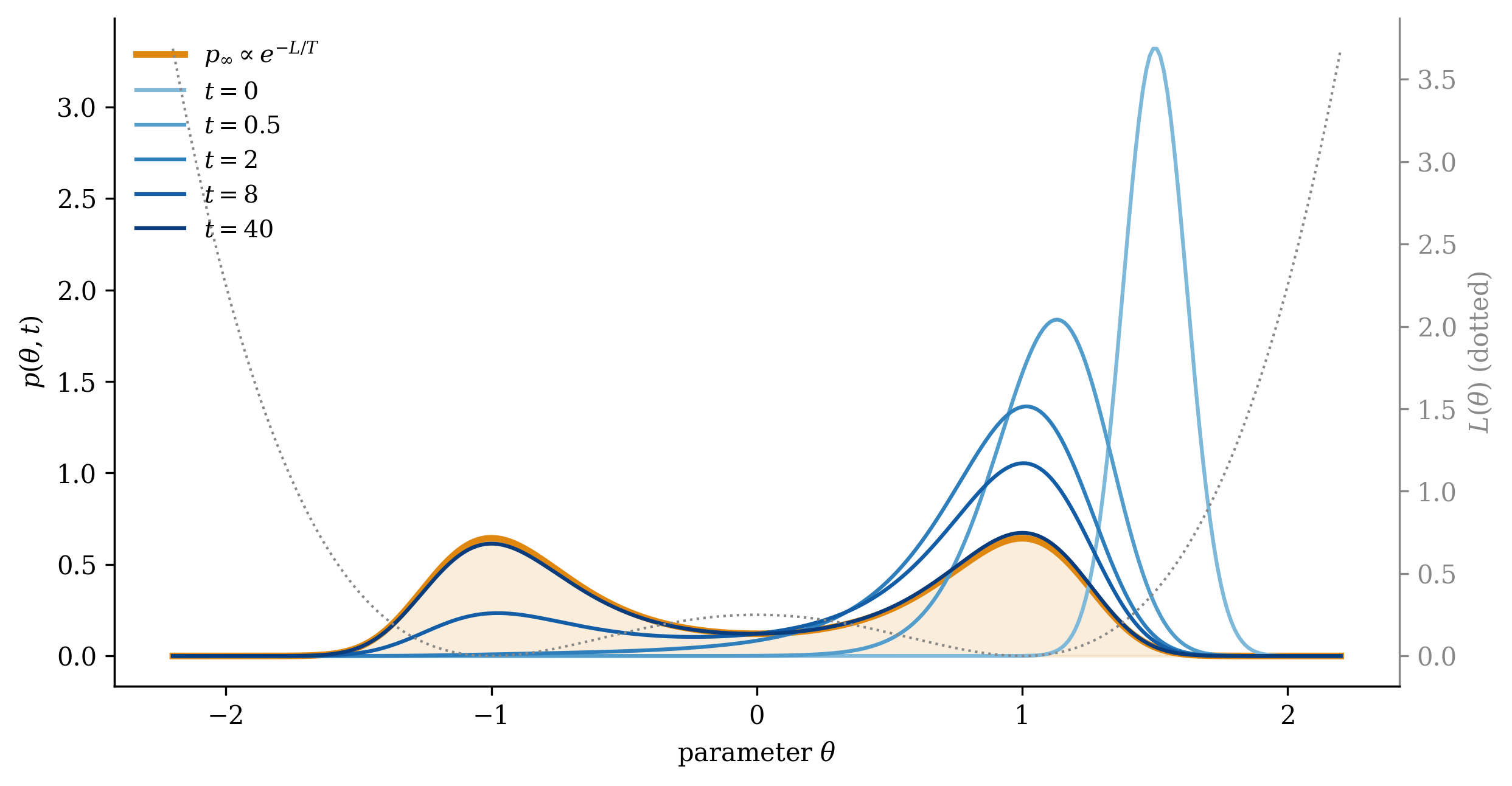
Figure 17.3 integrates Equation 17.3 numerically in a double-well loss and shows the full relaxation process: probability pours down the walls, thermalizes within the first well it finds, leaks across the barrier by diffusion, and settles onto \(e^{-L/T}\) — including the equal population of the second well that pure gradient descent, started on the right, would never touch.

Show code

T = 0.15
x = np.linspace(-2.2, 2.2, 331)
dx = x[1] - x[0]
dt = 0.25 * dx**2 / (2 * T)
L = 0.25 * (x**2 - 1) ** 2
Lp_mid = (0.5 * (x[1:] + x[:-1])) ** 3 - 0.5 * (x[1:] + x[:-1])

p = np.exp(-0.5 * ((x - 1.5) / 0.12) ** 2)       # start: all mass on the right wall
p /= p.sum() * dx
snap_times = [0.0, 0.5, 2.0, 8.0, 40.0]
snaps, t = {}, 0.0
while t <= snap_times[-1] + dt:
    for ts in snap_times:
        if ts not in snaps and t >= ts:
            snaps[ts] = p.copy()
    pm = 0.5 * (p[1:] + p[:-1])
    J = -pm * Lp_mid - T * (p[1:] - p[:-1]) / dx  # drift current + diffusion current
    p[1:-1] -= dt * (J[1:] - J[:-1]) / dx         # continuity: dp/dt = -dJ/dx
    t += dt

p_inf = np.exp(-L / T)
p_inf /= p_inf.sum() * dx

fig, ax = plt.subplots(figsize=(8.4, 4.4))
ax.fill_between(x, p_inf, color=ORANGE, alpha=0.15)
ax.plot(x, p_inf, color=ORANGE, lw=2.6, label=r"$p_\infty \propto e^{-L/T}$")
blues = plt.cm.Blues(np.linspace(0.45, 0.95, len(snap_times)))
for ts, col in zip(snap_times, blues):
    ax.plot(x, snaps[ts], color=col, lw=1.5, label=rf"$t = {ts:g}$")
ax2 = ax.twinx()
ax2.plot(x, L, color=GRAY, lw=1.0, ls=":")
ax2.set_ylabel(r"$L(\theta)$ (dotted)", color=GRAY, fontsize=10)
ax2.tick_params(axis="y", colors=GRAY)
ax2.spines["right"].set_visible(True)
ax2.spines["right"].set_color(GRAY)
ax.set_xlabel(r"parameter $\theta$")
ax.set_ylabel(r"$p(\theta, t)$")
ax.legend(frameon=False, fontsize=9.5, loc="upper left")
fig.tight_layout(); plt.show()

Figure 17.3: The Fokker–Planck equation Equation 17.3 solved numerically in the double-well loss \(L(\theta) = (\theta^2 - 1)^2/4\) (gray dotted, right axis) at \(T = 0.15\), starting from a narrow distribution on the right wall (\(t = 0\)). Drift pours the probability into the right well (\(t = 0.5\)), where it thermalizes to a local Boltzmann shape (\(t = 2\)); diffusion then carries mass over the barrier — height \(0.25 \approx 1.7\,T\) — into the left well (\(t = 8\)), until the current vanishes everywhere and the density settles onto the stationary Boltzmann law \(p_\infty \propto e^{-L/T}\) (orange): by \(t = 40\) the two agree to within \(5\%\), with \(0.478\) of the mass in the left well against the exact \(0.5\). Gradient descent started at the same point would sit at \(\theta = 1\) forever; the temperature explores both wells.

Take-home 2

The iterate’s distribution obeys the Fokker–Planck equation \(\partial_t p = \nabla \cdot (p \nabla L) + T \nabla^2 p\) — descent transporting probability against diffusion spreading it — and its equilibrium, where the probability current vanishes, is the Boltzmann distribution \(p_\infty \propto e^{-L/T}\) (Equation 17.4). SGD samples a Boltzmann distribution over the loss, thermalizing into a cloud of covariance \(T H^{-1}\) around a minimum rather than reaching it.

17.5 The temperature of training, and where the picture bends

What \(T \propto \eta/|B|\) buys. Three practical facts, previously empirical, are now one thermodynamic statement. First, the linear scaling rule of large-batch training — when you double the batch size, double the learning rate — is exactly the statement that only the ratio \(\eta/|B|\) matters: it holds the temperature fixed. Second, batch size is not thermodynamically neutral: growing \(|B|\) at fixed \(\eta\) cools the dynamics, which is why large-batch training converges sharply but explores little — a fact with generalization consequences that the next lecture takes up. Third, Week 8’s annealing schedules translate verbatim: decaying the learning rate during training is cooling this sampler, walking \(T \to 0\) so the stationary cloud contracts onto a minimum. The practitioner’s learning-rate schedule and the physicist’s cooling schedule are, by Equation 17.2, the same object — SGLD (Welling and Teh 2011) made that identification by design, adding calibrated isotropic noise; plain SGD arrives at it for free, with noise it already had.

Where it bends. The derivation of Equation 17.4 slipped in one assumption: isotropic noise, \(C = c I\), so that the diffusion is a scalar temperature. Real gradient noise fails this, structurally. The covariance \(C(\theta)\) is built from the data, varies across parameter space, and near minima aligns its large directions with the large-curvature directions of the loss — the noise kicks hardest exactly where the landscape is steepest. With an anisotropic diffusion tensor \(D\), the equilibrium condition \(J = 0\) requires \(\nabla L = -D\, \nabla \log p\), which demands that \(D^{-1} \nabla L\) be itself a gradient — and for generic \(D\) and \(L\) it is not. Then no distribution makes the current vanish: the best available stationary state has \(\nabla \cdot J = 0\) with \(J \neq 0\) — probability circulating forever, a non-equilibrium steady state, exactly the case anticipated by the distinction planted under Equation 17.3. Chaudhari and Soatto (2018) push this to its conclusion: for deep networks, SGD is out of equilibrium, its stationary distribution is not \(e^{-L/T}\) for any effective loss, and its dynamics can orbit in limit cycles rather than rest. The temperature picture survives as the leading, isotropic approximation — genuinely predictive, as the example below shows, and genuinely incomplete.

The near-minimum truth. One regime stays exactly solvable and gives the tutorial its target. Near a quadratic minimum, \(L \approx \frac{1}{2} \theta^{\mathsf{T}} H \theta\), the Langevin process is the Ornstein–Uhlenbeck process, and its stationary covariance \(\Sigma\) solves the Lyapunov equation

\[ H \Sigma + \Sigma H \;=\; 2 D, \qquad D = \frac{\eta\, C}{2 |B|}, \tag{17.5}\]

stationary covariance, general noise

which collapses to the Boltzmann answer \(\Sigma = T H^{-1}\) exactly when \(C \propto I\) and not otherwise. This equation — not the clean Boltzmann law — is what a measurement should be compared against, and measuring its ingredients is the tutorial’s assignment: estimate \(C(\theta)\) on a real network, check its isotropy, and test the predicted stationary cloud.

Trap

Three ways to misuse a temperature. ① The clean \(p_\infty \propto e^{-L/T}\) requires isotropic gradient noise. Real SGD noise is anisotropic and state-dependent, so the true stationary state solves Equation 17.5 near minima and is in general non-equilibrium, with persistent probability currents and no potential (Chaudhari and Soatto 2018) — do not claim SGD exactly samples \(e^{-L/T}\). ② Both knobs move \(T \propto \eta/|B|\): changing the batch size at fixed learning rate changes the temperature (the linear scaling rule compensates precisely this). ③ Today’s dynamics lives in parameter space — \(\nabla_\theta\), loss as energy — not the configuration-space \(\nabla_x\) of Weeks 10–12. The same Langevin/Fokker–Planck machinery runs in both spaces; the objects it moves are entirely different.

Take-home 3

\(T \propto \eta/|B|\) makes the learning rate and batch size two dials on one temperature: the linear scaling rule holds \(T\) fixed, large batches cool, and annealing the learning rate is cooling the sampler. But the Boltzmann law assumed isotropic noise — real gradient noise is anisotropic and state-dependent, the stationary covariance solves the Lyapunov equation \(H\Sigma + \Sigma H = 2D\) rather than \(T H^{-1}\), and in general SGD is a non-equilibrium process with persistent currents. The clean picture is the leading approximation; the tutorial measures the correction.

17.6 Example: SGD on a quadratic loss

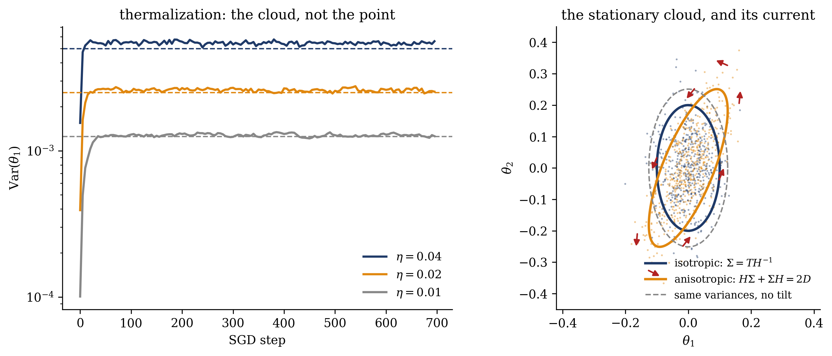
The exactly solvable case, simulated in full, tests every claim above against a number. Take \(L(\theta) = \frac{1}{2} \theta^{\mathsf{T}} H \theta\) in two dimensions with \(H = \mathrm{diag}(4, 1)\) — one steep direction, one flat — and run plain SGD with synthetic gradient noise of controllable covariance \(C\) (batch size absorbed into \(C\); \(T = \eta/2\) for unit isotropic noise). Figure 17.4 shows the two experiments.

The left panel is the thermalization claim. An ensemble of \(4000\) runs starts from a single point; the ensemble variance of \(\theta_1\) rises and then plateaus — the iterate has stopped converging and started sampling. The plateau sits where Equation 17.4 puts it, \(\mathrm{Var}(\theta_1) = T/\lambda_1\), and halving \(\eta\) halves it: measured \(0.00259\) and \(0.00128\) against predicted \(0.00250\) and \(0.00125\) for \(\eta = 0.02\) and \(0.01\). This is annealing in miniature: each cooler curve is the same algorithm with a smaller cloud. The hottest run shows the promised discreteness correction — measured \(0.00540\) against the SDE’s \(0.00500\), an \(8\%\) excess that the exact discrete-time calculation (\(\mathrm{Var} = \frac{T}{\lambda}\, \frac{2}{2 - \eta \lambda} = 0.00543\)) accounts for almost entirely: the Langevin picture is the small-\(\eta\) limit, and at \(\eta \lambda = 0.16\) the limit is already visibly approximate.

The right panel is the caveat made visible. With isotropic noise (navy) the stationary cloud matches the Boltzmann ellipse \(T H^{-1}\) — elongated along the flat direction, as Figure 17.1 promised. With anisotropic noise of the same average strength, tilted \(45°\) to the Hessian axes (orange), the cloud tilts too: its covariance matches the Lyapunov solution of Equation 17.5 (correlation \(0.71\) measured, \(0.72\) predicted) and no Boltzmann distribution — no function of \(L\) alone — has that shape, since any \(e^{-L/T}\) inherits the Hessian’s axes (gray dashed). The red arrows complete the diagnosis: the stationary current \(J = p \cdot (D \Sigma^{-1} - H)\, \theta\) does not vanish but circulates (its matrix has purely imaginary eigenvalues \(\pm 1.57 i\)) — probability orbiting the minimum forever, a non-equilibrium steady state in the smallest possible example. The effect visible in two dimensions persists in real networks; measuring it there is the tutorial’s work.

Show code

rng = np.random.default_rng(4)
lam = np.array([4.0, 1.0])                     # Hessian eigenvalues

fig, (a1, a2) = plt.subplots(1, 2, figsize=(10.4, 4.2))

# (a) thermalization: ensemble variance of theta_1 vs step, three temperatures
n_w, n_s, rec = 4000, 700, 5
for eta, col in [(0.04, NAVY), (0.02, ORANGE), (0.01, GRAY)]:
    th = np.tile([1.2, 1.2], (n_w, 1))
    steps, var1 = [], []
    for k in range(n_s):
        th += -eta * th * lam + eta * rng.standard_normal((n_w, 2))
        if k % rec == 0:
            steps.append(k)
            var1.append(th[:, 0].var())
    a1.semilogy(steps, var1, color=col, lw=1.8, label=rf"$\eta = {eta}$")
    a1.axhline(eta / 2 / lam[0], color=col, ls="--", lw=1.1)
a1.set_xlabel("SGD step")
a1.set_ylabel(r"$\mathrm{Var}(\theta_1)$")
a1.set_title("thermalization: the cloud, not the point", fontsize=11.5)
a1.legend(frameon=False, fontsize=9.5)

# (b) stationary clouds: isotropic vs anisotropic noise
def ellipse(S, nsig=2.0, n=200):
    w, V = np.linalg.eigh(S)
    ph = np.linspace(0, 2 * np.pi, n)
    return V @ (nsig * np.sqrt(w)[:, None] * np.vstack([np.cos(ph), np.sin(ph)]))

eta = 0.02
T_iso = eta / 2
ang = np.pi / 4
R = np.array([[np.cos(ang), -np.sin(ang)], [np.sin(ang), np.cos(ang)]])
C = R @ np.diag([3.0, 0.15]) @ R.T             # anisotropic, tilted 45 degrees
A = np.linalg.cholesky(C)
D = eta * C / 2
Sig_lyap = 2 * D / np.add.outer(lam, lam)      # solves H Sigma + Sigma H = 2D

n_w2, n_s2 = 6000, 6000
th_i = np.zeros((n_w2, 2))
th_a = np.zeros((n_w2, 2))
for _ in range(n_s2):
    th_i += -eta * th_i * lam + eta * rng.standard_normal((n_w2, 2))
    th_a += -eta * th_a * lam + eta * (rng.standard_normal((n_w2, 2)) @ A.T)

a2.plot(th_i[::12, 0], th_i[::12, 1], ".", color=NAVY, ms=1.2, alpha=0.4)
a2.plot(th_a[::12, 0], th_a[::12, 1], ".", color=ORANGE, ms=1.2, alpha=0.4)
e = ellipse(np.diag(T_iso / lam))
a2.plot(e[0], e[1], color=NAVY, lw=2.0, label=r"isotropic: $\Sigma = T H^{-1}$")
e = ellipse(Sig_lyap)
a2.plot(e[0], e[1], color=ORANGE, lw=2.0,
        label=r"anisotropic: $H\Sigma + \Sigma H = 2D$")
e = ellipse(np.diag(np.diag(Sig_lyap)))
a2.plot(e[0], e[1], color=GRAY, lw=1.2, ls="--", label="same variances, no tilt")

# the non-equilibrium circulation: v = J/p = (D Sigma^{-1} - H) theta
M = np.diag(lam) - D @ np.linalg.inv(Sig_lyap)
for ph in np.linspace(0, 2 * np.pi, 8, endpoint=False):
    pt = ellipse(Sig_lyap, nsig=2.6)[:, int(200 * ph / (2 * np.pi))]
    v = -M @ pt
    v *= 0.055 / np.linalg.norm(v)
    a2.annotate("", xy=pt + v, xytext=pt,
                arrowprops=dict(arrowstyle="-|>", color=RED, lw=1.3))
a2.set_xlabel(r"$\theta_1$")
a2.set_ylabel(r"$\theta_2$")
a2.set_xlim(-0.42, 0.42)
a2.set_ylim(-0.45, 0.45)
a2.set_aspect("equal")
a2.set_title("the stationary cloud, and its current", fontsize=11.5)
a2.legend(frameon=False, fontsize=8.5, loc="lower right")
fig.tight_layout(); plt.show()

Figure 17.4: SGD on the quadratic loss \(L = \frac{1}{2}\theta^{\mathsf{T}} H \theta\), \(H = \mathrm{diag}(4, 1)\) — the exactly solvable (Ornstein–Uhlenbeck) case. Left: ensemble variance of \(\theta_1\) over \(4000\) runs for three learning rates (isotropic noise). Each run thermalizes into a stationary cloud whose variance (plateau) matches the Boltzmann prediction \(T/\lambda_1\) with \(T = \eta/2\) (dashed): \(0.00259\) vs. \(0.00250\) at \(\eta = 0.02\), \(0.00128\) vs. \(0.00125\) at \(\eta = 0.01\); halving the learning rate halves the cloud (annealing in miniature). At \(\eta = 0.04\) the measured \(0.00540\) exceeds the SDE’s \(0.00500\) by the discrete-step correction \(2/(2 - \eta\lambda_1)\), giving \(0.00543\) — the Langevin limit is a small-\(\eta\) statement. Right: stationary clouds at \(\eta = 0.02\). Isotropic noise (navy points) fills the Boltzmann ellipse \(\Sigma = T H^{-1}\), axis-aligned and wide along the flat direction. Anisotropic noise of equal average strength, tilted \(45°\) (orange points), produces a tilted cloud matching the Lyapunov solution \(H\Sigma + \Sigma H = 2D\) (correlation \(0.71\) measured vs. \(0.72\) predicted) — a shape no \(e^{-L/T}\) can produce (gray dashed: the same variances without the tilt). Red arrows: the non-vanishing stationary current circulating around the minimum (eigenvalues \(\pm 1.57i\)) — non-equilibrium, in two dimensions.

17.7 Outlook: the measurement, the flat minima, and the reverse

The week continues from here. The warm-up card, due the evening before the next lecture, is unusually a recap: read the Ornstein–Uhlenbeck sections of Mandt, Hoffman, and Blei (2017) holding today’s derivation — the paper is this lecture in the notation of the field that rediscovered it. The tutorial (16–18, Ph12 106) takes the theory to the laboratory: measure the mini-batch gradient-noise covariance \(C(\theta)\) on a real network, test its isotropy, and compare the stationary fluctuations against Equation 17.5 — the prediction is on the table. The next lecture draws the consequence the whole picture has been pointing at: if training is sampling at a temperature, then the temperature decides which minima carry the stationary weight — wide, flat basins hold more Boltzmann mass than sharp ones of equal depth — and the flat-minima account of generalization, with entropy-SGD as its deliberate algorithmic version, follows.

The machinery extends well beyond this week. The Langevin equation and its Fokker–Planck companion are, in Week 10, transplanted from parameter space to configuration space — dynamics over data \(x\) rather than weights \(\theta\), where \(\nabla_x \log Z = 0\) removes Module 1’s obstruction outright — and in Week 12 they are run backwards in time: a diffusion that noises data into a Gaussian, inverted into a generative model. Every diffusion model is these equations, reversed — the road from sampling to generation runs through the same two boxed equations.

SGD is not descent — it is Langevin dynamics: training samples a Boltzmann distribution over the loss, and the learning rate is its temperature.