22 Annealed importance sampling: the equality becomes an estimator

22.1 From equality to estimator

The previous lecture proved an equality; this lecture turns it into an estimator. For any driven protocol, however fast and however irreversible, the work along stochastic trajectories satisfies \(\langle e^{-W} \rangle = e^{-\Delta F}\) — an exact statement where classical thermodynamics offered only the inequality \(\langle W \rangle \geq \Delta F\), with the Crooks theorem (Equation 21.3) standing behind it and the second law recovered as its Jensen shadow. (Throughout this lecture we absorb \(\beta\) into the energies, so the previous lecture’s \(\langle e^{-\beta W} \rangle = e^{-\beta \Delta F}\) (Equation 21.4) reads \(\langle e^{-W} \rangle = e^{-\Delta F}\); nothing is lost, and the symbols stay light.) The warm-up card sent you into Jarzynski’s four pages with the derivation already on the board, and the natural question to carry out of that reading is the one that organizes today: if every single run dissipates — if \(W > \Delta F\) on essentially every trajectory you will ever simulate — where does an exact equality live? The previous lecture’s answer was that it lives in the rare trajectories with \(W < \Delta F\), which the exponential average amplifies. That answer matters twice: it explains why the equality is useful, and it identifies the estimator’s practical limitation.

The equality addresses a problem the course has carried since Module 1, with three specific instances. Week 3 trained a restricted Boltzmann machine around its partition function — contrastive divergence dodges the negative phase — but flagged that the trained model’s log-likelihood was out of reach, because \(\log p(v) = \log f(v) - \log Z\) needs the one number training never produced (Section 6.4). Week 8 sharpened the complaint into a principle: MCMC samples \(p \propto e^{-E}\) precisely because \(Z\) cancels in every acceptance ratio, and for exactly that reason a chain can never deliver \(Z\) — samples are not normalizers (Section 15.4). Week 10 removed \(Z\) from training and from generation (Equation 19.1, Equation 20.2) but pointedly did not produce a number for it: a score-matched model has no likelihood to report. Three modules of machinery, and the course still cannot compare two energy-based models, report a free energy, or evaluate the RBM it trained nine weeks ago. All three require the same object the previous lecture’s theorem computes: a ratio of partition functions, \(Z_K/Z_0\), with the reference \(Z_0\) known in closed form.

The history has an unusual shape here. This course has repeatedly met results that waited decades for their application — Onsager’s 1936 reaction field for TAP, Bethe’s 1935 lattice approximation for belief propagation, Anderson’s 1982 reversal theorem for diffusion models. This week the pattern compresses to a year or so: Jarzynski (1997) proved the equality for driven Hamiltonian systems, and Neal (2001, circulated as a preprint in 1998) constructed the same identity inside Markov-chain Monte Carlo, as a variance repair of importance sampling, noting the correspondence to Jarzynski himself. Two fields arrived at one identity nearly simultaneously and met only afterwards. Neal’s construction is annealed importance sampling (AIS), and the task is to build the dictionary between the previous lecture’s physics and Neal’s algorithm, prove the algorithm exact by the same argument, and use Crooks to characterize its variance. Week 10 removed \(Z\) where it could be removed; Week 11 estimates it where it must be estimated.

22.2 One jump: importance sampling and its collapse

We start with the obvious attempt, because its failure dictates everything that follows. Suppose we can sample a tractable reference \(\pi_0 = f_0/Z_0\) (a Gaussian, independent spins — anything with \(Z_0\) in closed form) and we want the normalizer of a target \(\pi_K = f_K/Z_K\) of which we hold only the unnormalized \(f_K\). Importance sampling answers in one line: draw \(x \sim \pi_0\) and average the importance weight \(w = f_K(x)/f_0(x)\),

\[ \langle w \rangle_{\pi_0} = \int \mathrm{d}x\, \pi_0(x)\, \frac{f_K(x)}{f_0(x)} = \frac{1}{Z_0} \int \mathrm{d}x\, f_K(x) = \frac{Z_K}{Z_0} . \]

The estimator is unbiased for any \(\pi_0\) whatsoever, and it already has the previous lecture’s structure: for the instantaneous protocol that switches \(E_0 \to E_K\) in a single step, \(\log w = -[E_K(x) - E_0(x)] = -W\), and the display above is the Jarzynski equality (Equation 21.4) for the fastest possible driving. So where is the catch? Compute the second moment the same way:

\[ \langle w^2 \rangle_{\pi_0} = \int \mathrm{d}x\, \pi_0(x)\, \frac{f_K(x)^2}{f_0(x)^2} = \frac{Z_K^2}{Z_0^2} \int \mathrm{d}x\, \frac{\pi_K(x)^2}{\pi_0(x)} , \]

so that the relative variance is

\[ \frac{\mathrm{Var}[w]}{\langle w \rangle^2} = \int \mathrm{d}x\, \frac{\pi_K(x)^2}{\pi_0(x)} - 1 \;\equiv\; \chi^2(\pi_K \| \pi_0) , \tag{22.1}\]

relative variance of one-jump importance sampling

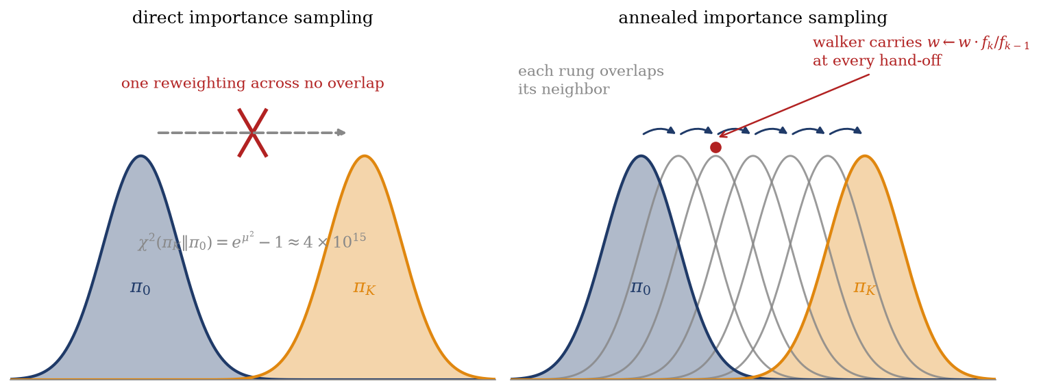
the chi-squared divergence between target and reference. The formula is exact, but its variance is severe: the integrand puts \(\pi_K^2\) over \(\pi_0\), so any region where the target has mass and the reference has almost none contributes enormously. For two unit Gaussians a distance \(\mu\) apart the integral closes — completing the square in \(\int \mathrm{d}x\, \mathcal{N}(x; \mu, 1)^2 / \mathcal{N}(x; 0, 1)\) leaves a factor \(e^{\mu^2}\) — giving \(\chi^2 = e^{\mu^2} - 1\). At \(\mu = 6\), a six-standard-deviation gap that any interesting target exceeds without trying, \(\chi^2 \approx 4 \times 10^{15}\).

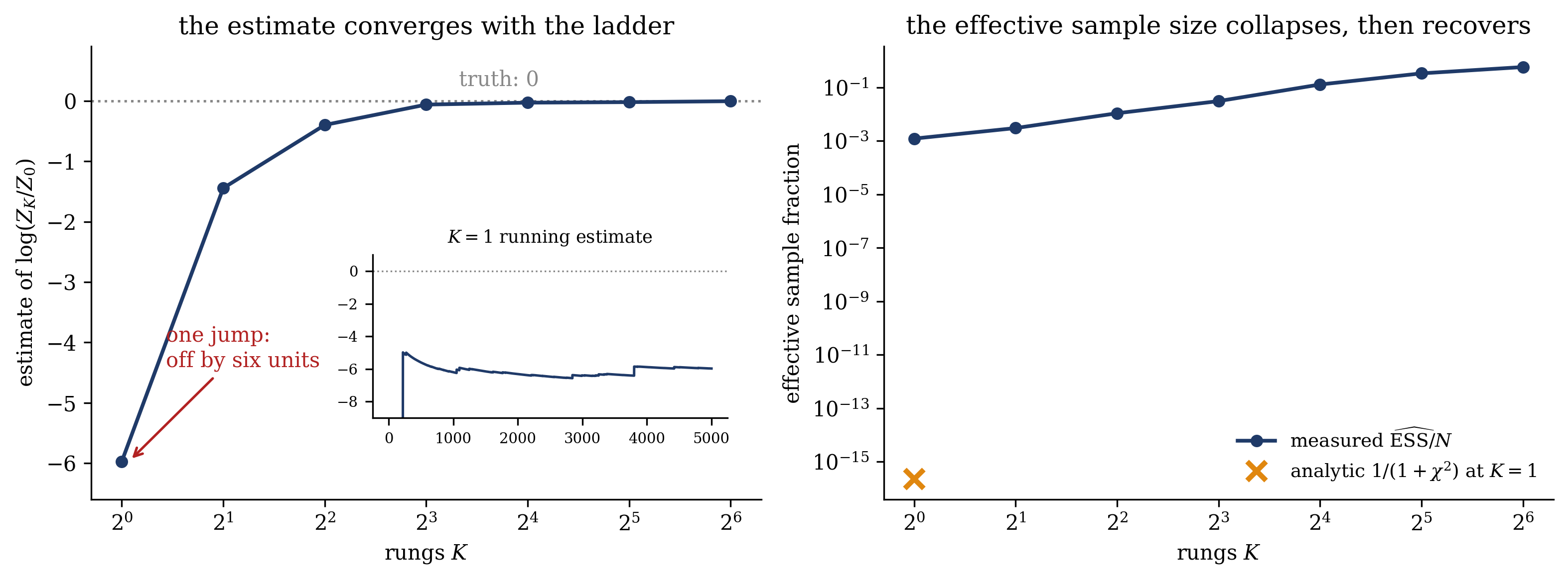
What that number costs in samples is made precise by the effective sample size: for self-normalized importance sampling, \(N\) draws from \(\pi_0\) carry the statistical weight of only \(\mathrm{ESS} = N/(1 + \chi^2)\) independent draws from the target, estimated in practice by \(\widehat{\mathrm{ESS}} = (\sum_i w_i)^2 / \sum_i w_i^2\). At \(\mu = 6\) and \(N = 10^4\), the effective sample size is of order \(10^{-12}\) — a trillionth of one sample. The estimator fails quantitatively, not conceptually: it is unbiased, yet unusable across any real gap.

Figure 22.1: The central picture of the lecture. Left: direct importance sampling attempts a single reweighting from the reference \(\pi_0\) to a target \(\pi_K\) six standard deviations away; the relative variance is the chi-squared divergence Equation 22.1, here \(e^{36} - 1 \approx 4 \times 10^{15}\), and the estimator collapses. Right: annealed importance sampling threads the same gap with a ladder of intermediate distributions, each overlapping its neighbor; a walker alternates weight updates (at the hand-offs between rungs, where \(w \leftarrow w \cdot f_k/f_{k-1}\)) with MCMC moves that need no normalizers. The mean of the accumulated weight is exact for any ladder; what the ladder buys is variance.

The repair is the previous lecture’s physics read backwards, and Figure 22.1 shows it before any formula does. A single switch dissipates severely; many gentle switches, each relaxed by a little dynamics, dissipate almost nothing. Thread the gap with a ladder of intermediate distributions, each overlapping its neighbor, and replace the one impossible reweighting by \(K\) easy ones. The claim that needs proof — and it is less obvious than the picture suggests — is that interleaving reweightings with MCMC moves leaves the estimator exactly unbiased, for any ladder and any number of rungs.

Take-home 1

Direct importance sampling estimates \(Z_K/Z_0\) without bias, with relative variance \(\chi^2(\pi_K \| \pi_0)\) — exponentially large in any real gap between reference and target (\(e^{\mu^2} - 1\) for unit Gaussians a distance \(\mu\) apart). Its logarithm is the previous lecture’s work for an instantaneous switch, and its failure is maximal dissipation seen from the estimator’s side. The repair is a ladder of intermediates: many small reweightings in place of one impossible one.

22.3 The ladder: switch, move, repeat

The intermediates come first. Between the reference \(f_0\) and the target \(f_K\) place the geometric path

\[ f_k(x) = f_0(x)^{1 - \beta_k}\, f_K(x)^{\beta_k}, \qquad 0 = \beta_0 < \beta_1 < \cdots < \beta_K = 1 , \]

with \(\pi_k = f_k/Z_k\). The annealing schedule \(\beta_k\) is a design choice, not a temperature — flag the clash once: \(\beta\) was an inverse temperature all course, and here it interpolates energies, \(E_k = (1 - \beta_k) E_0 + \beta_k E_K\). For a Boltzmann target with a flat reference the two readings coincide and the geometric path is the temperature ladder of Chapter 16 (Equation 16.4) — the same schedule that cooled to optimize in Week 8, now redeployed as a measuring instrument. Each \(\pi_k\) overlaps its neighbors by construction; the gap of Figure 22.1 has become \(K\) small steps.

The algorithm of Neal (2001) walks the ladder, alternating two elementary moves. Initialize \(x_0 \sim \pi_0\) (exact, since the reference is tractable) and \(w = 1\); then for \(k = 1, \ldots, K\):

① Switch. Multiply the weight by the ratio of adjacent rungs at the current configuration,

\[ w \;\leftarrow\; w \cdot \frac{f_k(x_{k-1})}{f_{k-1}(x_{k-1})} . \tag{22.2}\]

the AIS weight accumulates only at switches

② Move. Draw \(x_k\) from any Markov kernel \(T_k\) that leaves \(\pi_k\) invariant — a few Metropolis steps at rung \(k\), say. By Equation 15.2 the kernel needs only energy differences; every \(Z_k\) cancels, exactly as in Week 8.

Return \(w\) after the last switch. Two structural remarks before the theorem. First, where the record lives: the kernel steps contribute nothing to \(w\) — the entire history accumulates at the switches, and in the previous lecture’s dictionary the switch increment is precisely the work of moving the Hamiltonian under a frozen configuration, \(\log w = -\sum_{k=1}^{K} \left[ E_k(x_{k-1}) - E_{k-1}(x_{k-1}) \right] = -W\). The protocol has become a schedule, the trajectory a sequence of MCMC states, and the work an accumulated log-weight; the dictionary is complete. Second, what is never asked: the kernels are required to leave each \(\pi_k\) invariant, not to converge to it. A single Metropolis step per rung is legitimate, and no stage of the algorithm equilibrates. AIS is a transport with exact bookkeeping of its own irreversibility. The same structure appeared in Chapter 20 as the reverse-time SDE; here it takes discrete, weighted form. The next section proves the weight is unbiased.

22.4 The engine: importance sampling on whole paths

We prove that the accumulated weight is unbiased, \(\langle w \rangle = Z_K/Z_0\), for any schedule and any invariant kernels. The idea, due to Neal, is to apply ordinary importance sampling not on configurations but on the extended state space of whole annealing paths \((x_0, x_1, \ldots, x_{K-1})\) — and it is Jarzynski’s trajectory-ensemble argument in discrete time.

The forward path density. The algorithm itself defines a distribution over paths: draw from the reference, then apply the kernels in order,

\[ q_F(x_0, \ldots, x_{K-1}) = \pi_0(x_0)\, T_1(x_0 \to x_1)\, T_2(x_1 \to x_2) \cdots T_{K-1}(x_{K-2} \to x_{K-1}) . \]

The reverse path density. Define a second distribution on the same space by running the ladder from the far end: draw \(x_{K-1} \sim \pi_K\), then walk down with the reversed kernels,

\[ q_R(x_0, \ldots, x_{K-1}) = \pi_K(x_{K-1})\, \tilde{T}_{K-1}(x_{K-1} \to x_{K-2}) \cdots \tilde{T}_1(x_1 \to x_0) , \]

where \(\tilde{T}_k\) is the reversal of \(T_k\) with respect to its invariant distribution,

\[ \pi_k(x)\, T_k(x \to x') = \pi_k(x')\, \tilde{T}_k(x' \to x) . \]

The reversal is exactly the balance bookkeeping of Week 8: for a detailed-balance kernel (Equation 15.1) the two sides already match with \(\tilde{T}_k = T_k\), and Metropolis kernels are of this kind — but the proof needs only invariance, so we carry the general \(\tilde{T}_k\) (summing the definition over \(x\) confirms that \(\tilde{T}_k\) is a proper kernel precisely because \(\pi_k T_k = \pi_k\)).

The ratio telescopes. Now compute the importance-sampling ratio of the two path densities. Each substitution of the reversal definition trades a \(\tilde{T}_k\) for a \(T_k\) at the cost of a ratio of \(\pi_k\)’s:

\[ \begin{aligned} \frac{q_R(x_0, \ldots, x_{K-1})}{q_F(x_0, \ldots, x_{K-1})} &= \frac{\pi_K(x_{K-1})}{\pi_0(x_0)} \prod_{k=1}^{K-1} \frac{\tilde{T}_k(x_k \to x_{k-1})}{T_k(x_{k-1} \to x_k)} = \frac{\pi_K(x_{K-1})}{\pi_0(x_0)} \prod_{k=1}^{K-1} \frac{\pi_k(x_{k-1})}{\pi_k(x_k)} \\[2pt] &= \prod_{k=1}^{K} \frac{\pi_k(x_{k-1})}{\pi_{k-1}(x_{k-1})} = \prod_{k=1}^{K} \underbrace{\frac{Z_{k-1}}{Z_k}}_{\text{telescopes to } Z_0/Z_K}\, \frac{f_k(x_{k-1})}{f_{k-1}(x_{k-1})} = \frac{Z_0}{Z_K}\, w , \end{aligned} \]

where the second line regroups the same factors by configuration rather than by kernel — every \(\pi_k(x_k)\) in a denominator meets the \(\pi_k\) evaluated one step earlier in a numerator — and the normalizers of the interior rungs cancel in adjacent pairs. The ratio of two path measures is, pointwise, the AIS weight times a constant. Unbiasedness follows: since \(q_R\) is normalized on the extended space,

\[ \langle w \rangle_{q_F} = \int \mathrm{d}x_0 \cdots \mathrm{d}x_{K-1}\; q_F \cdot \frac{Z_K}{Z_0} \frac{q_R}{q_F} = \frac{Z_K}{Z_0} \underbrace{\int \mathrm{d}x_0 \cdots \mathrm{d}x_{K-1}\; q_R}_{=\,1} , \]

and we box the master result:

\[ \boxed{\; \Big\langle \prod_{k=1}^{K} \frac{f_k(x_{k-1})}{f_{k-1}(x_{k-1})} \Big\rangle_{q_F} = \frac{Z_K}{Z_0} \quad \text{for any schedule and any invariant kernels.} \;} \tag{22.3}\]

annealed importance sampling is exact in expectation (Neal 2001)

In words: the AIS weight is the density ratio of the reverse path measure to the forward one, so the estimator is ordinary importance sampling promoted from states to whole annealing histories — and the \(\chi^2\) that controls its variance is now a divergence between path measures, which the schedule can make small even when the endpoint divergence is astronomical. One further line closes the dictionary. Substitute \(f_k = e^{-E_k}\): the weight becomes \(\log w = -W\), the boxed equation reads \(\langle e^{-W} \rangle = e^{-\Delta F}\) (Equation 21.4, with \(\beta\) absorbed), and the extended state space — the previous lecture wrote its measures \(P_F\) and \(P_R\) — is Jarzynski’s trajectory ensemble under a different name. The previous lecture’s proof and Neal’s are one proof; a physicist met it as a statement about driven systems, a statistician as a variance repair, within a year of each other.

Take-home 2

AIS alternates weight switches and invariant MCMC moves along a ladder from reference to target; the accumulated weight satisfies \(\langle w \rangle = Z_K/Z_0\) exactly, for any schedule and any number of rungs (Equation 22.3) — proved by importance sampling on the space of whole annealing paths, which is Jarzynski’s argument in discrete time. The kernels never see a normalizer, and nothing equilibrates; the identity alone carries the result.

22.5 The price: dissipation is the error bar

The expectation is exact regardless of schedule; what varies with the schedule is the variance, and the previous lecture’s Crooks theorem governs it. Jensen, and the direction of the bias. The logarithm is concave, so \(\langle \log w \rangle \leq \log \langle w \rangle = \log (Z_K/Z_0)\): log-weights underestimate the log-normalizer on average, and a forward AIS run delivers a stochastic lower bound on \(\log Z_K\). The direction matters more than it seems. An energy-based model’s log-likelihood is \(\log p = \log f - \log Z\), so an underestimated \(\log Z\) overestimates the log-likelihood — AIS-evaluated models look systematically better than they are, and the bias shrinks only as the estimator’s variance does.

The gap is the dissipation, and the dissipation is a KL divergence. Averaging the log of the telescoped ratio under \(q_F\) gives the size of the Jensen gap exactly: \(\big\langle \log (q_F/q_R) \big\rangle_{q_F} = D_\mathrm{KL}(q_F \| q_R)\) on one side, and \(\log(Z_K/Z_0) - \langle \log w \rangle\) on the other. With \(\log w = -W\) and \(\Delta F = -\log(Z_K/Z_0)\) this is

\[ \boxed{\; \log \frac{Z_K}{Z_0} - \langle \log w \rangle = \langle W \rangle - \Delta F = \langle W_\mathrm{diss} \rangle = D_\mathrm{KL}(q_F \,\|\, q_R) \;} \tag{22.4}\]

bias in the log, dissipated work, and path-measure asymmetry are one number

— the previous lecture’s dissipation identity (Equation 21.5), rederived on the ladder. The estimator’s difficulty is a thermodynamic quantity: how irreversibly the ladder is traversed, measured as the divergence between the forward transport and its reversal. A reversible schedule (\(q_F = q_R\)) has zero gap and zero excess variance; everything the estimator suffers, it suffers in proportion to its own dissipation.

Variance, and the rare-trajectory warning made operational. The previous lecture located the exponential average in the rare low-work tail (Section 21.4); for the estimator this is not a curiosity but the failure mode. The variance of \(w\) grows exponentially with the dissipation (the one-jump limit Equation 22.1 is the extreme case), and a finite sample that has not yet visited the tail does not merely converge slowly — it produces a stable-looking, wrong answer, because the running mean sits quietly below the truth until the next tail event jerks it upward. Monitor the effective sample size \((\sum w_i)^2/\sum w_i^2\), never the running mean; and note that at severe dissipation even \(\widehat{\mathrm{ESS}}\) flatters, since the weights that would expose the degeneracy are exactly the ones not yet sampled. The worked example below shows both pathologies on a target whose answer is known.

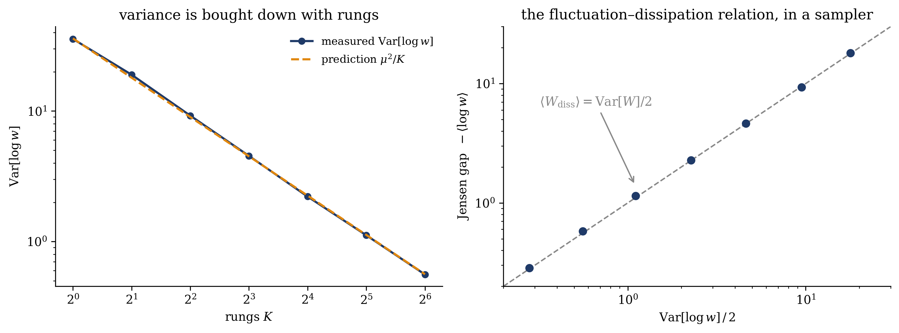
How fast does slowing down help? For a smooth schedule the dissipation obeys the near-equilibrium law \(\langle W_\mathrm{diss} \rangle \propto 1/K\): halving the per-rung jump quarters the per-rung dissipation (\(\chi^2\) per rung is quadratic in the jump) while doubling the rung count, for a net factor of one half. On the Gaussian ladder of the example this is elementary to verify — with well-mixed kernels the increment at rung \(k\) is \(\Delta\beta \, \mu (x - \mu/2)\) with \(x \sim \pi_{k-1}\), so each rung contributes variance \(\mu^2 \Delta\beta^2 = \mu^2/K^2\) and the total is \(\mathrm{Var}[\log w] \approx \mu^2/K\). And near equilibrium the work distribution is close to Gaussian, for which the Jarzynski equality itself fixes the relation between the two moments: \(e^{-\Delta F} = \langle e^{-W} \rangle = e^{-\langle W \rangle + \mathrm{Var}[W]/2}\), hence \(\langle W_\mathrm{diss} \rangle = \mathrm{Var}[W]/2\) — the fluctuation–dissipation relation for work, and a self-consistency check the example will display. Rungs are cheap insurance: the six-sigma gap that in one jump would need \(\sim 10^{15}\) raw draws to buy a single effective sample needs only \(K \gtrsim \mu^2\) rungs to bring \(\mathrm{Var}[\log w]\) to order one.

Further refinements belong in the record, each at a paragraph. The deterministic limit: as \(K \to \infty\) with perfect kernels, the sum of switch increments becomes \(\log (Z_K/Z_0) = \int_0^1 \mathrm{d}\beta\, \langle \partial_\beta \log f_\beta \rangle_{\pi_\beta}\) — thermodynamic integration, the quasistatic method Week 8 named alongside AIS (Section 15.4); AIS interpolates between free-energy perturbation (\(K = 1\)) and this limit, spending variance to save equilibration. Bidirectional estimators: running the ladder downward from the target gives a reverse weight whose Jensen bias has the opposite sign, so the pair brackets \(\log Z_K\) in a stochastic sandwich; combining both directions optimally is Bennett’s acceptance-ratio method (Bennett 1976), and reading \(\Delta F\) off the crossing of the forward and reverse work histograms is the previous lecture’s Crooks crossing, now as an estimator. When the answer matters, run both directions. Populations: running many walkers in parallel and occasionally resampling them by weight — killing the light, cloning the heavy — is sequential Monte Carlo, the population variant of AIS; we name it and move on.

The open problem of Week 3 is resolved in practice, not only in principle. Salakhutdinov and Murray (2008) ran exactly this machinery — a temperature ladder from the independent-unit RBM to the trained one, Gibbs transitions as the kernels — to put numbers on RBM partition functions and hence on the log-likelihoods that Section 6.4 declared unreachable; AIS has been the standard instrument for evaluating energy-based models since. Their caution is the Jensen paragraph above in the field’s own experience: the reported log-likelihoods are optimistic in expectation, and the direction of the bound belongs alongside the reported number.

Trap

The standard misreadings of an AIS run. ① Unbiased in \(Z\) is biased low in \(\log Z\). The mean of \(w\) is exact; the mean of \(\log w\) undershoots by exactly the dissipation (Equation 22.4) — and for model evaluation the sign flips into flattery, since a low \(\log Z\) inflates the log-likelihood. Report the direction of the bound with the number. ② A stable running mean is not convergence. The exponential average is carried by rare low-work paths; before the tail is sampled the estimate looks settled and is wrong, and at severe dissipation the ESS estimate is fooled with it. ③ The weight accumulates only at switches, and invariance is the only requirement. Kernel steps are weight-neutral (their \(Z_k\) cancels, Equation 15.2), and no rung equilibrates — accounting work into the MCMC moves, or demanding convergence at each rung, are the standard derivation errors. AIS is transport with exact bookkeeping, not a sequence of equilibrations.

Take-home 3

The Jensen gap \(\log(Z_K/Z_0) - \langle \log w \rangle\) equals the mean dissipated work, equals \(D_\mathrm{KL}(q_F \| q_R)\): bias in the log, variance, and thermodynamic irreversibility are one number (Equation 22.4). Forward AIS lower-bounds \(\log Z\) stochastically; slowing the schedule shrinks the gap as \(1/K\); near equilibrium \(\langle W_\mathrm{diss} \rangle = \mathrm{Var}[W]/2\). Budget rungs by dissipation, monitor the ESS rather than the running mean, and when the answer matters, run both directions.

22.6 Optimizing the reversal

We now look back at the engine’s proof with a designer’s eye. Unbiasedness needed very little from the reverse path density: \(q_R\) had to start at the target and be normalized — nothing more. The reversed kernels \(\tilde{T}_k\), built from the rungs’ invariant distributions, were Neal’s choice, not a requirement of the argument, and it is worth asking what the best choice would have been. The answer turns out to be Bayes’ rule, the proof is a one-line application of Week 10’s backward kernel, and the consequence — one week early — is the training objective of a diffusion model (Welling, Lu, and Holdijk 2026, ch. 12 on sequential importance sampling).

Unbiasedness survives any reversal. Replace the \(\tilde{T}_k\) by arbitrary backward kernels \(K_k\), normalized in their output (\(\int \mathrm{d}x_{k-1}\, K_k(x_k \to x_{k-1}) = 1\)), and define

\[ q_R^{(K)}(x_0, \ldots, x_{K-1}) = \pi_K(x_{K-1})\, \prod_{k=1}^{K-1} K_k(x_k \to x_{k-1}), \qquad w = \frac{f_K(x_{K-1})}{f_0(x_0)} \prod_{k=1}^{K-1} \frac{K_k(x_k \to x_{k-1})}{T_k(x_{k-1} \to x_k)} , \]

still computable on the fly — unnormalized densities and kernel evaluations only. Then \(w = (Z_K/Z_0)\, q_R^{(K)}/q_F\) pointwise, so the one-line argument of Section 22.4 gives \(\langle w \rangle_{q_F} = Z_K/Z_0\) unchanged, and the Jensen bookkeeping of Section 22.5 gives \(\langle \log w \rangle = \log(Z_K/Z_0) - D_\mathrm{KL}(q_F \| q_R^{(K)})\): the dissipation identity Equation 22.4 holds verbatim for the general reversal. (Substituting \(K_k = \tilde{T}_k\) collapses the kernel ratios through the reversal definition and recovers Equation 22.2, as it must.) Exactness is indifferent to how we reverse; the variance is not, and the reversal has become a design variable.

The optimal reversal is Bayes’ rule. Week 10 established that a forward Markov chain factorizes exactly through its own Bayes kernels (Equation 20.3). Applied to the annealing walker: write \(q_k\) for the marginal of the forward process after rung \(k\) — with \(q_0 = \pi_0\), and \(q_k \neq \pi_k\) in general, since the unequilibrated walker lags the ladder — and let \(B_k(x_k \to x_{k-1}) = T_k(x_{k-1} \to x_k)\, q_{k-1}(x_{k-1}) / q_k(x_k)\) be the true inverse of the transport actually run. Then \(q_F = q_{K-1}(x_{K-1}) \prod_k B_k(x_k \to x_{k-1})\), by the same two-line telescoping as in Week 10, and dividing this factorization by \(q_R^{(K)}\) splits the dissipation rung by rung:

\[ D_\mathrm{KL}\big(q_F \,\|\, q_R^{(K)}\big) = D_\mathrm{KL}\big(q_{K-1} \,\|\, \pi_K\big) + \sum_{k=1}^{K-1} \Big\langle D_\mathrm{KL}\big( B_k(x_k \to \cdot\,) \,\|\, K_k(x_k \to \cdot\,) \big) \Big\rangle_{q_k} . \tag{22.5}\]

the dissipation, resolved rung by rung

The first term is the lag — how far the transported reference \(q_{K-1}\) ends from the target — and does not involve the \(K_k\) at all. The second is a sum of nonnegative per-rung mismatches between the chosen reversal and the true inverse, so the minimum is immediate: set \(K_k = B_k\) and every summand vanishes. The variance-optimal reversal is Bayes’ rule applied to the nonequilibrium marginals of the transport, not the adjoint built on the rungs’ equilibria. At the optimum, moreover, the weight telescopes through the \(q_k\) and the entire interior of the path cancels, \(w = f_K(x_{K-1}) / \big(Z_0\, q_{K-1}(x_{K-1})\big)\): what remains is one-jump importance sampling (Equation 22.1) from \(q_{K-1}\) — the reference after it has been dragged across the gap — rather than from \(\pi_0\) across all of it. The exact denoiser repairs every rung’s dissipation in hindsight, and only the lag is left standing.

Why Neal’s algorithm does not use it. The kernel \(B_k\) requires the marginals \(q_k\) — the density of a driven, unequilibrated walker, an integral over its entire history, and precisely as intractable as the problem being solved. The adjoint \(\tilde{T}_k\) needs only ratios of the \(f_k\). AIS is therefore a deliberate trade — an evaluable reversal in place of the optimal one — and Equation 22.5 prices the trade exactly, at the per-rung mismatch between \(B_k\) and \(\tilde{T}_k\). Week 10 also says when that price vanishes: the backward kernel coincides with the adjoint precisely at stationarity, so \(B_k \to \tilde{T}_k\) as \(q_k \to \pi_k\) — the adiabatic regime, in which the kernels keep the walker equilibrated on every rung. Neal’s choice is the optimal reversal’s equilibrium approximation, and it improves exactly as fast as the schedule slows.

The third option is Week 12’s. Between the evaluable adjoint and the intractable Bayes inverse runs a middle road: learn the reversal. Parameterize the backward kernels and adjust them to minimize \(D_\mathrm{KL}(q_F \| q_R)\) — by Equation 22.5 a regression of each \(K_k\) toward the true denoiser \(B_k\), and by the generalized dissipation identity the same operation as maximizing the stochastic lower bound \(\langle \log w \rangle\) on \(\log(Z_K/Z_0)\): an evidence lower bound in the sense of Chapter 14, promoted from configurations to paths. That is a complete specification of the diffusion-model training problem, stated a week before the course builds one — fix a forward corruption, parameterize its reversal, minimize a forward–reverse path divergence — and it explains in advance why the object Week 12’s network regresses toward is a conditional Bayes kernel. What Week 12 adds is the Gaussian machinery that makes the regression tractable.

22.7 Example: a six-sigma gap, one jump versus sixty-four rungs

We now put numbers on the mechanism, on a target where every claim is checkable. Take \(\pi_0 = \mathcal{N}(0, 1)\) and \(\pi_K = \mathcal{N}(6, 1)\) — both endpoints normalized Gaussians, so the true answer is \(\log (Z_K/Z_0) = 0\) by construction and every error is visible. The geometric path between them is the mean-shift ladder \(\mathcal{N}(6\beta_k, 1)\) (up to a known factor absorbed in the \(f_k\)), the schedule is uniform, \(\beta_k = k/K\), and the kernels are twenty Metropolis steps of width one per rung. We run \(N = 5000\) walkers for \(K \in \{1, 2, 4, \ldots, 64\}\), with \(K = 1\) reproducing direct importance sampling across the full gap.

Show code

fig, (a1, a2) = plt.subplots(1, 2, figsize=(10.6, 4.0))

a1.axhline(0.0, color=GRAY, lw=1.2, ls=":")
a1.plot(Ks, lnZ_est, "o-", color=NAVY, lw=1.8, ms=5)
a1.set_xscale("log", base=2)
a1.set_ylim(-6.6, 0.9)
a1.set_xlabel(r"rungs $K$")
a1.set_ylabel(r"estimate of $\log(Z_K/Z_0)$")
a1.annotate("one jump:\noff by six units", xy=(1.05, lnZ_est[0]),
            xytext=(1.35, -4.4), color=RED, fontsize=10,
            arrowprops=dict(arrowstyle="->", color=RED, lw=1.2))
a1.text(10, 0.25, "truth: 0", color=GRAY, fontsize=10)
a1.set_title("the estimate converges with the ladder", fontsize=12)

ins = a1.inset_axes([0.42, 0.18, 0.53, 0.36])
lnw1 = runs[1]
m = lnw1.max()
w1 = np.exp(lnw1 - m)
running = m + np.log(np.cumsum(w1) / np.arange(1, len(w1) + 1))
ins.plot(np.arange(1, len(w1) + 1), running, color=NAVY, lw=1.2)
ins.axhline(0.0, color=GRAY, lw=0.8, ls=":")
ins.set_ylim(-9, 1)
ins.set_title(r"$K=1$ running estimate", fontsize=8.5)
ins.tick_params(labelsize=7)

a2.plot(Ks, ess_frac, "o-", color=NAVY, lw=1.8, ms=5,
        label=r"measured $\widehat{\mathrm{ESS}}/N$")
a2.plot([1], [2.3e-16], "x", color=ORANGE, ms=9, mew=2.5,
        label=r"analytic $1/(1+\chi^2)$ at $K=1$")
a2.set_xscale("log", base=2)
a2.set_yscale("log")
a2.set_xlabel(r"rungs $K$")
a2.set_ylabel("effective sample fraction")
a2.legend(frameon=False, fontsize=9, loc="lower right")
a2.set_title("the effective sample size collapses, then recovers", fontsize=12)
fig.tight_layout()
plt.show()

Figure 22.2: One jump versus the ladder, on the six-sigma Gaussian gap (\(\pi_0 = \mathcal{N}(0,1)\), \(\pi_K = \mathcal{N}(6,1)\), true \(\log(Z_K/Z_0) = 0\); \(N = 5000\) walkers, 20 Metropolis steps of width 1 per rung, fixed seed). Left: the AIS estimate of \(\log(Z_K/Z_0)\) against the rung count \(K\). Direct importance sampling (\(K = 1\)) sits at \(-5.97\), six units below the truth; by \(K = 64\) the estimate is \(-0.006\). The inset shows the \(K = 1\) running estimate against sample count: it drifts through \(-6.2\) at \(N = 1000\) and \(-6.0\) at \(N = 5000\), settled-looking throughout and wrong by six units — the tail that carries the mean has not been sampled, and nothing in the trace says so. Right: the measured effective-sample-size fraction \(\widehat{\mathrm{ESS}}/N\) (navy); at \(K = 1\) it reports about \(6\) usable walkers of \(5000\), while the analytic value \(1/(1+\chi^2) = 2.3 \times 10^{-16}\) (orange cross) shows the estimator for the diagnostic is itself fooled by thirteen orders of magnitude.

The left panel of Figure 22.2 shows the mechanism numerically. One jump lands at \(-5.97\) against a true value of \(0\), and its running mean (inset) would pass any casual convergence check while doing so — the second pathology of Section 22.5, demonstrated explicitly. The ladder walks the estimate onto the truth: \(-0.03\) by \(K = 16\) and \(-0.006\) at \(K = 64\), at a total cost of \(64 \times 20\) kernel steps per walker. The right panel prices the same story in effective samples, and adds the sharper warning: at \(K = 1\) the measured ESS reports six usable walkers where the analytic answer is \(10^{-12}\) of one — the diagnostic collapses exactly when it is needed most, because the weights that would expose the degeneracy live in the unsampled tail.

Show code

fig, (a1, a2) = plt.subplots(1, 2, figsize=(10.6, 4.0))

a1.plot(Ks, var_lnw, "o-", color=NAVY, lw=1.8, ms=5,
        label=r"measured $\mathrm{Var}[\log w]$")
a1.plot(Ks, MU**2 / Ks, "--", color=ORANGE, lw=1.8, label=r"prediction $\mu^2/K$")
a1.set_xscale("log", base=2)
a1.set_yscale("log")
a1.set_xlabel(r"rungs $K$")
a1.set_ylabel(r"$\mathrm{Var}[\log w]$")
a1.legend(frameon=False, fontsize=9)
a1.set_title("variance is bought down with rungs", fontsize=12)

lims = [0.2, 30]
a2.plot(lims, lims, "--", color=GRAY, lw=1.2)
a2.plot(var_lnw / 2, gap, "o", color=NAVY, ms=6)
a2.set_xscale("log")
a2.set_yscale("log")
a2.set_xlim(lims); a2.set_ylim(lims)
a2.set_xlabel(r"$\mathrm{Var}[\log w]\,/\,2$")
a2.set_ylabel(r"Jensen gap $\;-\langle \log w \rangle$")
a2.annotate(r"$\langle W_{\mathrm{diss}} \rangle = \mathrm{Var}[W]/2$",
            xy=(1.1, 1.4), xytext=(0.32, 6.5), color=GRAY, fontsize=10.5,
            arrowprops=dict(arrowstyle="->", color=GRAY, lw=1.1))
a2.set_title("the fluctuation–dissipation relation, in a sampler", fontsize=12)
fig.tight_layout()
plt.show()

Figure 22.3: Dissipation under schedule control, same runs as Figure 22.2. Left: the variance of the log-weight falls as the predicted \(\mu^2/K = 36/K\) (dashed) once the ladder resolves the gap — measured \(0.56\) at \(K = 64\) against the predicted \(0.5625\). Right: the measured Jensen gap \(-\langle \log w \rangle\) against half the log-weight variance, one point per \(K\); the points collapse onto the diagonal (\(0.285\) versus \(0.280\) at \(K = 64\)), which is the work fluctuation–dissipation relation \(\langle W_\mathrm{diss} \rangle = \mathrm{Var}[W]/2\) observed inside a sampler.

Figure 22.3 closes the loop on the theory of Section 22.5. The log-weight variance tracks \(\mu^2/K\) once the rungs resolve the gap (\(0.56\) measured against \(0.5625\) predicted at \(K = 64\)), so the six-sigma gap that defeated one jump is tamed by \(K \approx \mu^2\) gentle ones, as the near-equilibrium law promised. And the right panel is a piece of statistical mechanics observed inside an algorithm: the Jensen gap — the bias of the log-estimate, per Equation 22.4 the mean dissipated work — equals half the work variance, point by point along the schedule. The fluctuation–dissipation relation has become a convergence diagnostic.

Averages of \(W\) obey an inequality, but averages of \(e^{-W}\) obey an equality — and an equality is an estimator: the \(Z\) this course could never compute is the mean of an annealing weight.

The tutorial (16–18, Ph12 106) is computation-led, and the machinery is now complete: the weight recursion Equation 22.2, the unbiasedness result Equation 22.3, and the dissipation accounting Equation 22.4. The hard problem computes a free-energy difference by AIS on a target whose answer you do not know by symmetry, and verifies the Jarzynski equality numerically along the way; today’s example showed the failure mode and the scaling so that the tutorial can watch for both — the ESS estimator and the Jensen gap are the relevant diagnostics. The estimator is run by the groups, one machine each, on a prediction committed beforehand.

22.8 Outlook: from measuring transports to learning them

Week 11 completes the course’s treatment of the partition function. The spine has been \(Z\) since Week 1: dodged by Hopfield’s dynamics, bounded by mean field, cancelled by Metropolis, removed from training and generation by the score. Each of those was a way of not needing the number. This week the course computed it — from unequilibrated, finite-time, deliberately irreversible runs, with the previous lecture’s equality guaranteeing the mean and today’s dissipation accounting pricing the fluctuations. The three open problems from the introduction are resolved: RBM likelihoods (the instrument of Salakhutdinov and Murray (2008)), free-energy differences, and model comparison all reduce to \(Z\)-ratios, and \(Z\)-ratios are means of annealing weights.

The last step of the arc is no longer a measurement but a design problem, and Section 22.6 has already posed it. A diffusion model is a learned annealing path: the forward corruption of Section 20.2 is the ladder, the reverse-time SDE of Equation 20.2 is the transport, and the training loss that makes the reversal learnable is exactly the program that section wrote down — a Kullback–Leibler divergence between a forward and a reverse path measure, a dissipation minimized by gradient descent over the reversal. The lineage is the historical record: Sohl-Dickstein et al. (2015) built the first diffusion models directly from this literature, and their title — Deep Unsupervised Learning using Nonequilibrium Thermodynamics — is a citation of this week. Week 12 assembles the industrial object, DDPM and the score-SDE (Ho, Jain, and Abbeel 2020; Song et al. 2021), the previous lecture quantified the cost of nonequilibrium transport, today that cost became an estimator, and next week a neural network learns the transport that minimizes it.