27Synthesis: thirteen weeks, one variational principle
Recommended reading
Core (light — this lecture derives one identity and reads the course off it).Jaynes (1957) §1–4, re-read. The paper that Week 1 leaned on for the maximum-entropy derivation of Equation 1.2 is also the origin of today’s frame: the Boltzmann distribution as the solution of a variational problem, with everything else a consequence. Alongside it, Welling, Lu, and Holdijk (2026) — the companion text tells the same story this lecture tells, from the free-energy face rather than the \(Z\) face, and reading the two voices against each other is the best preparation for the exam’s translation questions.
Optional (retrospective pointers, not new reading). The Gibbs–Bogoliubov section of Week 5 (Section 9.3) — the engine below was met there as a tool; today it is the frame. The ELBO identity (Equation 9.2) and its VAE incarnation (Equation 14.6). The six-station spine figure of Week 12 (Figure 24.4), which today’s central picture completes. Tishby, Pereira, and Bialek (1999) — the seventh stance.
Prerequisite reminder. Everything the course boxed. New content: none — the work of this lecture is to show that the identity \(F = -T \log Z\) and the variational free energy \(F[q]\) were the hidden subject of all thirteen weeks, and to leave behind the one map the exam is organized around.
27.1 The whole map
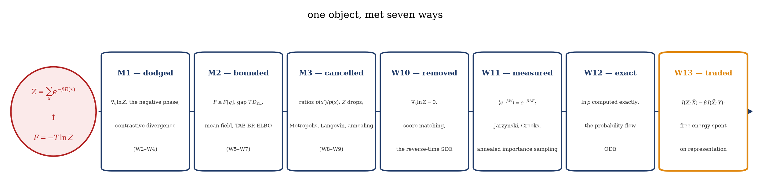
Week 1 opened with a thesis: statistical physics supplied machine learning with much of its modeling and inferential machinery, and the course would demonstrate the claim method by method. Thirteen weeks later the demonstration is complete, and it faces the standard risk of any demonstration by cases — that it reads as a catalog. We built energy-based memories, a variational toolbox, samplers, a nonequilibrium theory of generative models, and an information-theoretic coda, and each module closed with its own boxed results. The question a good physics course must answer at the end is whether these are thirteen techniques or one idea worked out thirteen times. The organizing object is the partition function \(Z = \sum_x e^{-\beta E(x)}\), easy to write and generally hard to compute. The course’s modules are not merely about \(Z\) — they are a sequence of stances toward it, and the sequence has a logic. Figure 27.1 draws it, extending the six-station figure that closed Week 12 (Figure 24.4) by the station Module 5 added.
Figure 27.1: One object, met seven ways: the completed spine of the course. Module 1 dodged the obstruction — the negative phase \(\nabla_\theta \log Z\) of Equation 5.5 blocked maximum-likelihood training, and contrastive divergence sidestepped it with a short chain (Week 3). Module 2 bounded it: \(F \leq F[q]\) for every trial distribution, with mean field, TAP, belief propagation, and the ELBO as four choices of family (Weeks 5–7). Module 3 cancelled it inside Metropolis ratios and Fokker–Planck stationary measures, at the price of mixing time (Weeks 8–9). Week 10 removed it from the learning problem altogether, since \(\nabla_x \log Z = 0\). Week 11 measured it, delivering \(\log Z\) as a nonequilibrium free-energy difference. Week 12 made the likelihood exact through the probability-flow ODE. Week 13 traded it: free energy spent on representation under an information constraint. The red ellipse is the claim of Section 27.5 — the two faces at the left are one object.
The map also settles a motif the course has used once per module and never yet named as a theme. Four times, a statistical-physics result sat in the literature for decades until machine learning needed it: Onsager’s reaction field of 1936 (Onsager 1936) became the TAP correction of spin-glass theory (Thouless, Anderson, and Palmer 1977) and then the stabilizing term of approximate message passing (Week 6); Bethe’s 1935 superlattice approximation (Bethe 1935) became belief propagation’s free energy (Yedidia, Freeman, and Weiss 2003); Anderson’s 1982 reverse-time diffusion theorem (Anderson 1982) became the generative half of every diffusion model (Week 10); and Jarzynski’s 1997 work relation (Jarzynski 1997) became annealed importance sampling (Neal 2001) and, structurally, the diffusion training objective (Weeks 11–12). The pattern is the practical content of the course’s thesis: the infrastructure transfers because the problem transfers — a Boltzmann distribution with an intractable normalizer is the same mathematical object whether \(x\) is a spin configuration or an image, and results proved about the object travel with it.
27.2 Two faces of one object
Before the derivation, we state the claim it will earn. The course has appeared to run on two rails. The narrative rail is \(Z\): the normalization that made Boltzmann-machine training intractable (Equation 5.5), the constant that Metropolis ratios cancel (Equation 15.2), the term whose configuration-gradient vanishes for score matching (Equation 19.1). The methodological rail is the free energy: Module 2 minimized a variational \(F[q]\), Week 8 cooled one, Week 11 measured differences of one, Week 13 constrained one. The two rails are connected by an identity the course has carried since its first lecture,
\[
\boxed{\; F \;=\; -\,T \log Z \;=\; \langle E \rangle - T\,S, \;}
\tag{27.1}\]
the two faces of the spine
The identity is an identification: there was never a second object. Whenever a week led with \(Z\), it was because the obstruction was easiest to point at on that face; whenever a week led with \(F\), it was because the variational structure was easiest to state there.
Week 1 obtained the Boltzmann distribution Equation 1.2 by maximizing the entropy \(S = -\sum_x p(x) \log p(x)\) at fixed mean energy (Jaynes 1957) — a variational statement. Since our entropies are in nats (\(k_B = 1\)), the \(S\) of that derivation is simultaneously the information entropy of Week 13; there is no conversion factor anywhere in the course. The whole spine therefore descends from one variational principle, and the engine below is that principle run in reverse: instead of maximizing entropy to find\(p\), we minimize free energy to approach it.
Take-home 1
The partition function and the free energy are one object seen two ways, \(F = -T \log Z\). The course’s modules are seven stances toward it — dodge, bound, cancel, remove, measure, make exact, trade — and Figure 27.1 is the whole course on one line.
27.3 The engine: the variational free energy, promoted
Week 5 met the Gibbs–Bogoliubov bound as the license for mean-field theory, derived it (Equation 9.1), and spent a module exploiting it. What Week 5 could not yet say is what the bound would become: the single inequality that every subsequent method of the course either tightens, saturates, or sidesteps. We therefore derive it once more, as the frame rather than the tool.
A notation panel, once, since the exam spans all of it. The trial distribution is \(q\) throughout — always the variational object, never a data distribution — and we write \(F[q]\) for what Week 5 called \(F_q\), to emphasize that it is a functional on distributions. The letter \(T\) is a temperature again (Week 12’s use of \(T\) as the diffusion horizon is retired), and the course has now used three distinct \(\beta\)’s: the thermal \(\beta = 1/T\) of every module, the noise schedule \(\beta_t\) of the diffusion weeks, and the information-bottleneck trade-off multiplier \(\beta\) of Week 13. They are cousins — each one prices a constraint — but they are not equal, and confusing them is the fastest route to a wrong exam answer. Sums over \(x\) carry over to integrals \(\int \mathrm{d}x\) everywhere, as they have since Module 3.
For any distribution \(q(x)\), define the variational free energy by transplanting the equilibrium formula \(F = \langle E \rangle - TS\) onto the trial state:
\[
F[q] \;=\; \langle E \rangle_q \;-\; T\,S[q]
\;=\; \sum_x q(x)\,E(x) \;+\; T \sum_x q(x) \log q(x).
\]
The target of every inference problem in this course is the Boltzmann distribution \(p(x) = e^{-\beta E(x)}/Z\) (Equation 1.2). Inverting it expresses the energy in terms of the target, \(E(x) = -T\big[\log p(x) + \log Z\big]\), and substituting into \(F[q]\) is the entire derivation:
\[
\begin{aligned}
F[q]
&= -\,T \sum_x q(x) \big[ \log p(x) + \log Z \big] \;+\; T \sum_x q(x) \log q(x) \\[2pt]
&= -\,T \log Z \, \underbrace{\sum_x q(x)}_{=\,1} \;+\; T \sum_x q(x) \log \frac{q(x)}{p(x)} \\[2pt]
&= -\,T \log Z \;+\; T\, D_\mathrm{KL}(q \,\|\, p).
\end{aligned}
\]
The Kullback–Leibler term is nonnegative — Gibbs’ inequality, which deserves its two lines now that it carries the course: since \(\log u \leq u - 1\) with equality only at \(u = 1\),
with equality if and only if \(q = p\) everywhere. Combining the two displays gives the master result:
\[
\boxed{\; F[q] \;=\; -\,T \log Z \;+\; T\, D_\mathrm{KL}(q \,\|\, p) \;\;\geq\;\; -\,T \log Z \;=\; F[p], \qquad \text{equality iff } q = p. \;}
\tag{27.2}\]
the course’s equation: Gibbs–Bogoliubov, promoted to the frame
⇒ The variational free energy of any trial state sits above the true free energy by exactly \(T\) times the information-theoretic distance to the target — the approximation error of a variational method is not vague; it is a KL divergence you can name before you compute anything.
Equation 27.2 admits three readings. Read as a bound, it says \(\log Z \geq -F[q]/T\): any tractable \(q\) yields a certificate on the log-partition function, which is Module 2. Read as an objective, it says that minimizing \(F[q]\) over a family simultaneously tightens the bound and finds the family member closest to \(p\) in KL — the dual role that connects magnetism (Week 5) with Bayesian inference (Week 7). Read as a limit, it says the floor is reached only at \(q = p\) itself: a method that insists on zero gap must produce the exact Boltzmann distribution, which is what sampling does and why Module 3 exists.
Take-home 2
\(F[q] = -T \log Z + T\,D_\mathrm{KL}(q\|p) \geq -T \log Z\), with equality iff \(q = p\) (Equation 27.2). Minimizing \(F\) over a restricted family bounds \(\log Z\) and the gap is exactly \(T\,D_\mathrm{KL}\); saturating the bound is exact sampling; and any method that only ever differentiates \(\log p\) with respect to \(x\) never sees \(Z\) at all. This single line organizes the course.
27.4 The seven-way read-off
Every method the course built is a specialization of Equation 27.2 — a choice of what family \(q\) may live in, and of what is held fixed while \(F[q]\) is pushed down. Table 27.1 sets them side by side; each circled entry below references the boxed result of its home lecture. It cuts finer than the seven verbs of Figure 27.1 rather than matching them one-to-one — bound fans out into mean field, BP, and the ELBO, and cancel into MCMC and annealing — and its first row restores Module 1’s contrastive divergence, the lone dodge whose gap is a truncation bias rather than a controlled KL. No new mathematics appears below.
Table 27.1: Every method is a choice of family for \(q\) and of what is held fixed in \(F[q]\); its approximation error is a KL divergence that can be named in advance.
method (home)
the family for \(q\)
held fixed
the gap \(T\,D_\mathrm{KL}(q\|p)\) is
contrastive divergence (W3)
the chain’s law after \(k\) steps from data
\(k\) Gibbs sweeps, data start
a truncation bias — not a controlled bound
mean field, TAP (W5–W6)
products \(\prod_i q_i(x_i)\)
\(E\), \(T\)
the discarded correlations
belief propagation (W6)
pair-consistent beliefs on a graph
the factor graph
the loop corrections
ELBO, VAE (W5, W7)
amortized \(q_\phi(z \mid x)\)
data \(x\), decoder
the posterior + amortization gap
MCMC (W8–W9)
states reachable by a chain in finite time
the target \(p\)
transient — it decays at the mixing rate
simulated annealing (W8)
the equilibria \(p_T\) along a schedule
\(E\)
zero at each rung; the schedule pays instead
score matching, diffusion (W10–W12)
reverse-path measures \(P_R^\theta\)
the forward noising \(P_F\)
the dissipation \(\beta(\langle W \rangle - \Delta F)\)
information bottleneck (W13)
encoders \(q(\tilde{x} \mid x)\)
the source \(p(x, y)\)
relevant information left uncaptured
① Mean field and TAP (Weeks 5–6). Restrict \(q\) to a product \(\prod_i q_i(x_i)\) and minimize: stationarity gives the self-consistency equations Equation 9.3, and the gap \(T\,D_\mathrm{KL}\) is exactly the correlation structure the factorization cannot carry — largest near criticality, where correlations are long-ranged, which is why mean field fails worst there. TAP (Equation 11.2) does not change the family; it corrects the functional, adding the Onsager reaction term as the next order of the Plefka expansion (Plefka 1982), and Week 6’s AMP transplanted the same correction to compressed sensing.
② Belief propagation (Week 6). Widen the family from single-site products to locally consistent pair beliefs and replace \(F\) by its Bethe approximation (Equation 12.3): the stationary points are exactly the fixed points of the message-passing equations (Yedidia, Freeman, and Weiss 2003). On a tree the Bethe free energy is the true \(F\) and the gap closes; on loopy graphs the loops are the gap.
③ The ELBO (Weeks 5 and 7). Transcribing Equation 27.2 to a Bayesian posterior gives Equation 9.2: the evidence lower bound is \(-F[q]\), so maximizing a likelihood bound is minimizing a free energy, term for term (Equation 14.6). The VAE’s amortized family \(q_\phi(z \mid x)\) makes the minimization a single neural-network pass (Kingma and Welling 2014), and its training curve is a free-energy descent whose remaining height above \(-\log p(x)\) is a KL (Equation 14.1).
④ MCMC (Weeks 8–9). Refuse any restriction and demand the saturating \(q = p\): detailed balance (Equation 15.1) builds a chain whose stationary state is exactly the Boltzmann distribution, with \(Z\) cancelling in every acceptance ratio (Equation 15.2). The bound’s slack is traded for a new price, the mixing time — the wall did not fall; it moved from bias to variance-per-unit-time. Week 9 read SGD itself in this column: a discretized Langevin equation whose stationary measure (Equation 17.4), for isotropic noise, is a Boltzmann distribution on weight space — real SGD noise is anisotropic and generically out of equilibrium (Chaudhari and Soatto (2018)), so the identification is the leading approximation, not an equality.
⑤ Simulated annealing (Week 8). Hold the family at the exact equilibria \(p_T\) and move the temperature: in \(F = \langle E \rangle - TS\), high \(T\) weights the entropy (broad, easy to sample) and \(T \to 0\) concentrates all probability on the energy minima (Equation 16.1) (Kirkpatrick, Gelatt, and Vecchi 1983). The gap is zero at every rung; what costs instead is the schedule, since cooling faster than the mixing time of ④ quenches into metastable states (Figure 16.1).
⑥ Score matching and diffusion (Weeks 10–12). Differentiate the logarithm with respect to configuration and \(Z\) leaves the problem: \(\nabla_x \log p = -\beta \nabla_x E\) (Equation 19.1), the training target that needs no normalizer, and Anderson’s reverse SDE (Equation 20.2) turns the learned score into a generator. The variational structure returns on trajectories: the DDPM objective (Equation 23.3) is Equation 27.2 written on path space, its gap the dissipation \(\beta(\langle W \rangle - \Delta F) = D_\mathrm{KL}(P_F \| P_R)\) of the fluctuation theorems (Equation 21.5, via Equation 21.4 and Equation 21.3). The same machinery settles Module 3’s debt — Jarzynski/AIS deliver \(\log Z\) itself as an average over driven paths (Equation 21.1, Equation 22.3) — and Week 12’s probability-flow ODE completes the arc with an exact likelihood (Equation 24.2).
⑦ The information bottleneck (Week 13). Constrain the minimization by an information budget: the IB Lagrangian (Equation 25.1) is a free energy with mutual informations in the roles of energy and entropy, its multiplier \(\beta\) a trade-off inverse temperature, and its self-consistent solution a Boltzmann distribution over codewords built on the rate–distortion free energy Equation 25.3. The seventh stance spends free energy on representation rather than generation — the same functional, pointed at a different question.
27.5\(Z\) and \(F\) were never two
The read-off resolves two questions that have recurred since Week 1. The first asked whether the spine of the course is the partition function or the variational free-energy principle. The question was malformed: by Equation 27.1 they are the same object, and the course simply used whichever face made the current obstruction visible — \(Z\) when the problem was normalization, \(F\) when the method was variational. The second asked whether the course has one recurring obstruction or two, since normalization blocks training (Module 1) while sampling hardness blocks estimation (Module 3). These are also one wall seen from two sides: if \(Z\) were cheap, \(p\) could be normalized and sampled directly; if \(p\) were cheap to sample, \(Z\) could be estimated by the free-energy methods of Week 11; and both statements are the assertion that \(F[q]\) is hard to push to its floor. The bound of Module 2, the sampler of Module 3, and the removal of Module 4 are three escapes from the same wall, priced respectively in bias (a KL gap), in time (mixing), and in scope (the score gives generation and likelihood, but never a thermodynamic potential unless Week 11’s machinery is added).
\(Z\) and the free energy were never two spines — \(F = -T \log Z\), and every method the course built either bounds \(F\) over a family, samples the \(q = p\) that saturates the bound, or removes \(Z\) by differentiating a logarithm. Thirteen weeks were one variational principle.
27.6 Example: the whole course on one landscape
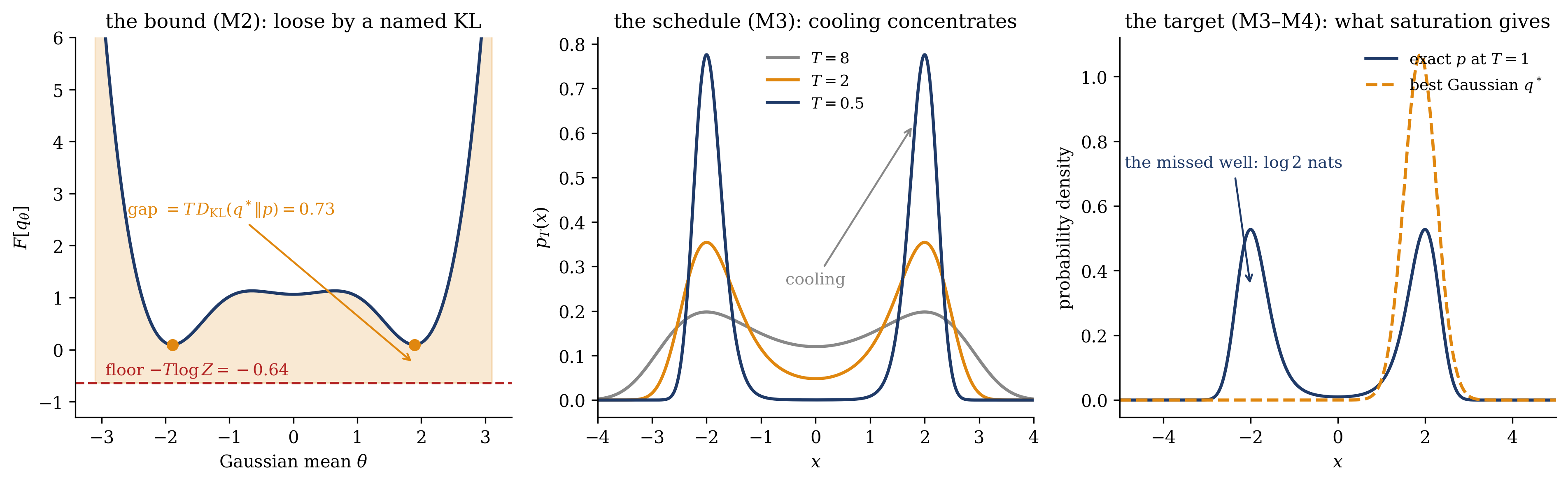
The synthesis fits in a single executable figure, and we build it from the course’s recurring stage set: a bistable energy, the continuous cousin of the two-mode target that Modules 3 and 4 sampled all semester. Take the double well \(E(x) = (x^2 - a^2)^2/4\) with \(a = 2\), so the wells sit at \(x = \pm 2\) and the barrier is \(4\) (in units of \(T\) at \(\beta = 1\)). Everything below is deterministic grid quadrature — no sampling, so every number is exact to plotting accuracy and the whole cell runs in seconds. We compute the floor \(-T \log Z\) once, then put three stances on it: the bound of Module 2, evaluated for the family of single Gaussians \(q_{\theta} = \mathcal{N}(\theta, \sigma^2)\) with \(\sigma\) optimized at each mean \(\theta\) (the moments of a quartic energy under a Gaussian are analytic, so \(F[q_\theta]\) needs no integrals at all); the cooling of Module 3, as the exact Boltzmann distribution \(p_T\) along a temperature ladder; and the target itself, which the sampling and score routes reach and the restricted family cannot.
Figure 27.2: The whole course on one free-energy landscape (double well \(E(x) = (x^2 - a^2)^2/4\), \(a = 2\), barrier \(= 4T\) at \(T = 1\); deterministic grid quadrature). Left: the variational free energy \(F[q_\theta]\) of the best Gaussian \(\mathcal{N}(\theta, \sigma^2(\theta))\) against its mean \(\theta\), with the exact floor \(-T\log Z = -0.640\) (red dashed) and the gap \(T\,D_\mathrm{KL}(q_\theta \| p)\) shaded. The bound Equation 27.2 holds everywhere; the best single Gaussian (\(\theta^* = \pm 1.89\), \(\sigma^* = 0.37\)) stops \(0.734\) nats above the floor — \(\log 2 = 0.693\) of that gap is the well the ansatz cannot represent, the remaining \(0.041\) the shape mismatch inside the well it keeps. The variational landscape is itself a double well: the restricted family breaks the symmetry it cannot describe, as mean field did in Week 5. Center: the exact Boltzmann \(p_T \propto e^{-E/T}\) at \(T = 8, 2, 0.5\) — cooling concentrates the target onto its wells (the barrier-to-well probability ratio falls from \(0.61\) to \(3\times 10^{-4}\)), the annealing mechanism of Equation 16.1, with the mixing price of Week 8 hiding in the vanishing weight between the wells. Right: at \(T = 1\), the exact bimodal target (navy) against the best single Gaussian (orange dashed) — the panel-left gap made visible as the missing mode, which the sampling route (Week 8) and the score route (Weeks 10 and 12) recover because neither restricts the family.
Figure 27.2 is the semester in three panels, and its numbers are exact enough to check by hand. The left panel is Week 5’s projection made quantitative on a target where we can check everything: the best product-family member stops at \(F[q^*] = 0.095\), which is \(0.734\) nats above the floor \(-T \log Z = -0.640\), and the decomposition of that gap is exact — a bimodal target approximated by a unimodal family costs at least the \(\log 2 = 0.693\) nats of the abandoned mode, and the measured excess of \(0.041\) nats is the residual shape mismatch between a Gaussian and one quartic well. (Week 5’s small-lattice experiment in Section 9.6 found the same anatomy on the Ising model.) The variational curve \(F[q_\theta]\) is itself a double well in \(\theta\) with a maximum at the symmetric point: the restricted family cannot straddle both modes, so it spontaneously breaks the symmetry — the pitchfork of Equation 9.3 and Equation 10.1, reappearing uninvited in a one-parameter fit, and a reminder that the mean-field magnet, the two-cluster posterior of Week 13’s block model, and this toy all order for the same reason. The center panel is the annealing mechanism with no algorithm attached: the exact minimizer of \(F[q]\) at each temperature is \(p_T\) itself, broad and barrier-crossing at \(T = 8\), essentially two disconnected wells by \(T = 0.5\) — and the vanishing of the between-well weight is exactly why Week 8’s chains mix exponentially slowly when quenched. The right panel is what the unrestricted stances deliver: MCMC (Week 8) and the learned score with its reverse SDE (Weeks 10 and 12) both target the navy curve, both wells included, because neither method ever wrote down a family — one saturates the bound by construction, the other bypasses \(Z\) by differentiation. The mixture \(0.7\,\mathcal{N}(-3, 0.5^2) + 0.3\,\mathcal{N}(3, 0.5^2)\) that served as Week 10’s standing target is this panel with unequal wells.
Trap
Four ways to lose the synthesis on the exam. ① The bound runs opposite to the ELBO by a sign.\(F[q] \geq -T\log Z\) is minimized; the ELBO \(= -F[q]\) is maximized and lower-bounds the log-evidence (Equation 9.2). They are the same inequality read from opposite faces — keep the convention \(p \propto e^{-\beta E}\) fixed and state which face you are on before manipulating signs. ② The gap is a KL divergence, not hand-waving. “Mean field is approximate” means precisely \(F[q] - F[p] = T\,D_\mathrm{KL}(q\|p) \geq 0\), computable in principle and computed above (\(0.734\) nats); an answer that treats the error as unquantifiable has missed the point of Equation 27.2. ③ Saturation is not free. Reaching \(q = p\) exactly (Module 3) exchanges the bound’s bias for mixing time; on the landscape above, the same barrier that starves the between-well weight is what traps the sampler. ④ Removed is not measured. Score matching makes \(Z\) irrelevant because \(\nabla_x \log Z = 0\) (Equation 19.1); it does not deliver \(\log Z\). Producing the number took Week 11’s work relations (Equation 21.1) — the stances “removed” and “measured” are distinct stations of Figure 27.1, and collapsing them is a category error.
Take-home 3
On one double-well landscape, the variational bound is visibly loose for a single-Gaussian family (a gap of \(0.734\) nats, of which \(\log 2\) is the missed mode), tightens to the floor only at \(q = p\), and is walked downhill by cooling \(T\) — mean field, annealing, and the exact target are three readings of one figure, and the figure is Equation 27.2 drawn.
27.7 The bridge out: the exam, the frontier, and the title
This week the tutorial machinery changes shape for the first time since Week 1: there is no hard problem and no warm-up card — the stuck-point sequence ended at Week 13 — and both the next lecture and tutorial slots are review. The next lecture is the structured exam preparation: question-driven, with two or three derivations walked end to end in the format the written exam expects, drawing on the accumulated tutorial problems of Weeks 1–13, reused and extended in the exam’s pattern. The 16–18 session continues the same work. The exam itself tests computational reasoning on that corpus — interpret a result, predict an output, locate the flaw — and it is organized around exactly the scaffold this lecture boarded: for any method you are handed, say what \(q\) it optimizes, what family \(q\) is restricted to, what is held fixed, and what the gap \(T\,D_\mathrm{KL}\) is — then you have located it on Table 27.1 and on Figure 27.1, and the rest is Weeks 2 through 13. The exam is closed-book, with any formula it needs but does not expect you to memorize printed on the paper, so that question set is also the recommended architecture for revision: the stances table, filled in with your own boxed results, is one page, and it is the page to know.
Alongside the \(Z\) spine, a second thread ran the length of the semester — phase transitions in learning systems: the capacity \(\alpha_c\) at which memory shatters (Equation 4.6), the \(T_c\) at which mean field orders (Equation 10.1), the convergence boundaries of message passing, and finally Week 13’s detectability threshold (Equation 26.4), where the thread became the subject. That is the course’s live frontier, surveyed in Section 26.7: neural-tangent-kernel and feature-learning theory (Jacot, Gabriel, and Hongler 2018), random-matrix analyses of learning curves, the spin-glass picture of deep loss landscapes (Choromanska et al. 2015), and the statistical-physics-of-inference programme (Zdeborová and Krzakala 2016). Those pointers, together with the free-energy synthesis of Welling, Lu, and Holdijk (2026), are where a student of this course can start doing research with the toolkit rather than learning it.
The title of the course names the route from Boltzmann to diffusion: the Boltzmann distribution \(e^{-\beta E}/Z\) entered as a modeling choice (Week 1, Equation 1.2); its normalizer blocked learning (1985) and was dodged (2002), bounded (1977–2014, from TAP to the VAE), and cancelled (1953); differentiating its logarithm removed it (2005); reversing its relaxation generated data (1982, used 2015–2021); driving it out of equilibrium measured it (1997); a change of variables made its likelihood exact (2021); and constraining its free energy by information turned the same machinery into a theory of representation (1999) and of solvability itself (2011). Every arrow in Figure 27.1 carries such a date, and most of the dates precede the applications by decades. Statistical physics is not an analogy for machine learning but its working infrastructure — and the infrastructure, as Module 5 showed, is still producing.
Bethe, Hans A. 1935. “Statistical Theory of Superlattices.”Proceedings of the Royal Society of London A 150 (871): 552–75. https://doi.org/10.1098/rspa.1935.0122.
Chaudhari, Pratik, and Stefano Soatto. 2018. “Stochastic Gradient Descent Performs Variational Inference, Converges to Limit Cycles for Deep Networks.” In International Conference on Learning Representations (ICLR).
Choromanska, Anna, Mikael Henaff, Michael Mathieu, Gérard Ben Arous, and Yann LeCun. 2015. “The Loss Surfaces of Multilayer Networks.” In AISTATS 2015, PMLR, 38:192–204.
Jacot, Arthur, Franck Gabriel, and Clément Hongler. 2018. “Neural Tangent Kernel: Convergence and Generalization in Neural Networks.” In NeurIPS. Vol. 31.
Kingma, Diederik P., and Max Welling. 2014. “Auto-Encoding Variational Bayes.” In International Conference on Learning Representations (ICLR).
Kirkpatrick, Scott, C. Daniel Gelatt, and Mario P. Vecchi. 1983. “Optimization by Simulated Annealing.”Science 220 (4598): 671–80. https://doi.org/10.1126/science.220.4598.671.
Onsager, Lars. 1936. “Electric Moments of Molecules in Liquids.”Journal of the American Chemical Society 58 (8): 1486–93. https://doi.org/10.1021/ja01299a050.
Plefka, Timm. 1982. “Convergence Condition of the TAP Equation for the Infinite-Ranged Ising Spin Glass Model.”Journal of Physics A: Mathematical and General 15 (6): 1971–78. https://doi.org/10.1088/0305-4470/15/6/035.
Thouless, David J., Philip W. Anderson, and Richard G. Palmer. 1977. “Solution of ’Solvable Model of a Spin Glass’.”Philosophical Magazine 35 (3): 593–601. https://doi.org/10.1080/14786437708235992.
Tishby, Naftali, Fernando C. Pereira, and William Bialek. 1999. “The Information Bottleneck Method.” In Proc. 37th Allerton Conference on Communication, Control, and Computing, 368–77.
Welling, Max, Sirui Lu, and Lars Holdijk. 2026. Generative AI and Stochastic Thermodynamics: A Tale of Free Energies. Cambridge: Cambridge University Press. https://doi.org/10.1017/9781009709071.
Yedidia, Jonathan S., William T. Freeman, and Yair Weiss. 2003. “Understanding Belief Propagation and Its Generalizations.” In Exploring Artificial Intelligence in the New Millennium, edited by Gerhard Lakemeyer and Bernhard Nebel, 239–69. San Francisco: Morgan Kaufmann.
Zdeborová, Lenka, and Florent Krzakala. 2016. “Statistical Physics of Inference: Thresholds and Algorithms.”Advances in Physics 65 (5): 453–552. https://doi.org/10.1080/00018732.2016.1211393.