20 The reverse-time SDE: generation is time reversal

20.1 Almost a generator

The previous lecture left one step between the learned score and a full generative model; this lecture supplies it. The score \(\nabla_x \log p = -\nabla_x E\) is free of the partition function, and Hyvärinen’s objective — in its denoising form especially — fits it from data alone. And Week 9 supplied the reason a score field should be worth fitting: the score is a drift. Langevin dynamics \(\mathrm{d}x = \nabla_x \log p(x)\,\mathrm{d}t + \sqrt{2}\,\mathrm{d}W\) has \(p\) as its stationary law (the configuration-space twin of Section 17.4’s parameter-space result), so a learned score plus a Langevin integrator is, in principle, a machine that turns noise into samples — almost a generator. (The warm-up card asked you to reverse an Ornstein–Uhlenbeck process, and it separates two questions: what the marginals of the reversed process must be, which Week 9 answers, and what dynamics achieves them, which is another matter entirely. That missing dynamics is today’s boxed theorem, and in the tutorial you will build the special case by hand.)

The qualification matters. Langevin sampling equilibrates: started anywhere, it must run until it forgets its initialization — and that is Module 3’s mixing problem again, in a new setting. On a multimodal target, the walker crosses between modes at exponentially rare intervals (Section 15.4; the trapped walker of Section 15.2), and knowing the score does not lower a single barrier — the drift field is precisely what builds the barrier. Worse, a second failure is specific to the learned setting: score matching trains \(s_\theta\) where the data live; in the low-density region between modes — exactly the terrain a mixing walker must cross — the learned score is unconstrained by any training signal, and the walker is steered by noise of our own manufacture. The worked example below makes the first failure quantitative in its purest form: with the exact score in hand and a generous step budget, Langevin on a two-mode target simply keeps whatever mode weights its initialization happened to have. Equilibrium sampling did not get easier because the previous lecture removed \(Z\).

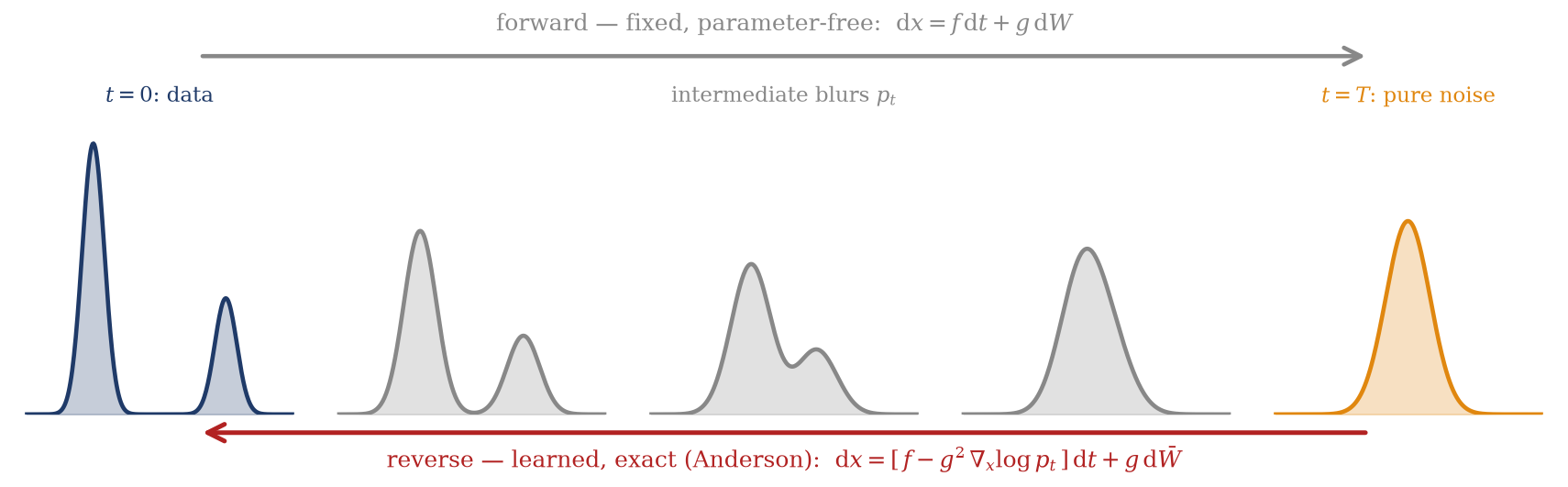
The fix is the founding idea of this module: do not equilibrate — transport. Take the one distribution in the problem that requires no mixing whatsoever — pure Gaussian noise — and manufacture a path from the data to it: a fixed, parameter-free forward diffusion that corrupts data to noise. Then reverse time. That the reversal exists — that a diffusion run backwards is again a diffusion, with a drift correction given exactly by the score of the time-marginals — is a theorem, proved by Anderson (1982) in the control-theory literature, forty years before generative modeling needed it (a recurring pattern in this course: Onsager 1936 waited for TAP, Bethe 1935 for belief propagation, Anderson 1982 for diffusion models). Generation becomes the corruption run in reverse, steered by the previous lecture’s \(Z\)-free score (Figure 20.1) — and the mixing problem is not solved but never encountered, because the reverse path starts at the only distribution that is already mixed and travels only through blurred intermediates whose barriers have melted.

Figure 20.1: The central picture of the lecture — a diffusion model as a film run twice. Top row (forward, left to right): a fixed noising SDE corrupts samples of the data density (navy, two unequal modes) through blurred intermediates \(p_t\) into a unit Gaussian — parameter-free, trivial to simulate, and the endpoint requires no mixing whatsoever. Bottom row (reverse, right to left): Anderson’s reverse-time SDE, steered by the score of each intermediate blur, carries fresh noise back through the *same* marginals to the data. Every panel of the bottom row is a distribution that the previous lecture’s denoising score matching was trained on; the barrier of the leftmost panel is never crossed, because the reverse path visits it only in its melted forms.

Take-home 1

A learned score plus Langevin is almost a generator — defeated by mixing (barriers between modes, unpriced by knowing the score) and coverage (the score is untrained exactly where a mixing walker must travel). The fix is nonequilibrium: corrupt data to noise with a fixed forward diffusion — noise needs no mixing — and reverse time, which Anderson’s theorem makes exact.

20.2 The forward process: corruption is easy

Everything today runs on one humble SDE. Take the Ornstein–Uhlenbeck (variance-preserving) forward process

\[ \mathrm{d}x \;=\; -x\,\mathrm{d}t \;+\; \sqrt{2}\,\mathrm{d}W \tag{20.1}\]

the forward (noising) process

— Week 9’s workhorse, now applied to data: start \(x_0 \sim p_0\) (the data distribution) and let every sample decay toward the origin while being kicked by noise. Its transition law is one line of Week 9 algebra (the script keeps it): \(x_t \mid x_0 \sim \mathcal{N}\!\big(x_0\,e^{-t},\; 1 - e^{-2t}\big)\). Three facts about the resulting time-marginals \(p_t\) follow:

The endpoint is free. As \(t\) grows, the memory of \(x_0\) decays as \(e^{-t}\) and the variance saturates: \(p_T \to \mathcal{N}(0, 1)\) for \(T\) of a few units, whatever the data were. The far end of the path is a unit Gaussian — exactly sampleable, no chain, no mixing, no \(Z\). Corruption is the one direction in which everything is easy.

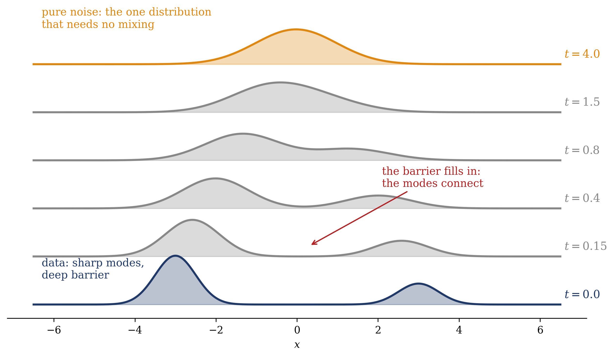
The intermediates are blurs, and the barrier vanishes. For each \(t\), \(p_t\) is the data smeared with a known Gaussian (a mixture of Gaussians stays a mixture: means shrink as \(e^{-t}\), widths grow toward one). Figure 20.2 computes the whole family exactly for a two-mode target: the sharp bimodal density at \(t = 0\) merges, hump by hump, into the unit Gaussian. Compare this picture with Langevin’s failure — the deep valley between the modes, the barrier that equilibration must cross, simply fills in along the path. A process that travels through the \(p_t\) in sequence never faces the \(t=0\) barrier at all.

The intermediates are where the score is trained. The previous lecture’s denoising score matching (Equation 19.4) fits \(s_\theta\) on noise-perturbed data — which is to say, on samples of precisely these \(p_t\). The regions a reverse-time path will travel through are, by construction, the regions where the learned score has seen data. Both of Langevin’s failures — barriers and coverage — are dissolved by the same corruption.

Show code

xs = np.linspace(-6.5, 6.5, 500)
ts = [0.0, 0.15, 0.4, 0.8, 1.5, 4.0]
fig, ax = plt.subplots(figsize=(8.6, 5.0))
for k, t in enumerate(ts):
    y = pt_density(xs, t)
    base = 0.55 * k
    col = NAVY if t == 0 else (ORANGE if t == ts[-1] else GRAY)
    ax.fill_between(xs, base, base + y, color=col, alpha=0.30)
    ax.plot(xs, base + y, color=col, lw=2.0)
    ax.text(6.6, base + 0.05, rf"$t = {t}$", color=col, fontsize=11, va="bottom")
ax.annotate("the barrier fills in:\nthe modes connect", xy=(0.3, 0.55 * 1 + 0.12),
            xytext=(2.1, 1.35), color=RED, fontsize=10.5,
            arrowprops=dict(arrowstyle="->", color=RED, lw=1.2))
ax.text(-6.3, 0.55 * 5 + 0.42, "pure noise: the one distribution\nthat needs no mixing",
        color=ORANGE, fontsize=10.5)
ax.text(-6.3, 0.30, "data: sharp modes,\ndeep barrier", color=NAVY, fontsize=10.5)
ax.set_xlabel(r"$x$")
ax.set_yticks([])
ax.spines["left"].set_visible(False)
fig.tight_layout(); plt.show()

Figure 20.2: The barrier melts. Exact time-marginals \(p_t\) of the running two-mode data density (\(0.7\,\mathcal{N}(-3, 0.5^2) + 0.3\,\mathcal{N}(3, 0.5^2)\)) under the forward process Equation 20.1, drawn bottom to top — a Gaussian mixture stays a Gaussian mixture, with means shrinking as \(e^{-t}\) and widths saturating, so every curve is closed-form. The deep valley between the modes — the barrier that blocks equilibrium sampling at \(t = 0\) — fills in within half a time unit, and by \(t = 4\) the marginal is a unit Gaussian, indistinguishable from noise. A process that travels through these blurs in sequence never confronts the \(t=0\) barrier; that process is the subject of the next section.

20.3 The engine: the reverse-time SDE

Corrupting is trivial; the question is whether the corruption can be reversed. Precisely: does there exist a stochastic process, run from \(t = T\) backwards to \(t = 0\), whose time-\(t\) marginals are the same \(p_t\) as the forward corruption — so that starting it from cheap noise delivers, at \(t = 0\), genuine samples of the data? We derive the answer with machinery the course already owns: Week 9’s Fokker–Planck equation, read with fresh eyes.

Step 1 — the marginal flow, recalled. The forward SDE \(\mathrm{d}x = f(x,t)\,\mathrm{d}t + g(t)\,\mathrm{d}W\) (our case: \(f = -x\), \(g = \sqrt{2}\)) transports its marginals according to the Fokker–Planck equation of Equation 17.3:

\[ \partial_t\, p_t \;=\; -\nabla_x \!\cdot\! \big( f\, p_t \big) \;+\; \tfrac{g^2}{2}\, \nabla_x^2\, p_t \]

— a drift current plus diffusive spreading.

Step 2 — the central rewrite. The diffusion term is secretly a drift term. Since \(\nabla_x p_t = p_t\, \nabla_x \log p_t\) — the score, converting a density gradient into a transport velocity — we can write \(\tfrac{g^2}{2} \nabla_x^2 p_t = \nabla_x \cdot \big( \tfrac{g^2}{2} (\nabla_x \log p_t)\, p_t \big)\), and the whole Fokker–Planck equation collapses into a single probability current:

\[ \partial_t\, p_t \;=\; -\nabla_x \!\cdot\! \Big[ \Big( \underbrace{f - \tfrac{g^2}{2} \nabla_x \log p_t}_{\text{effective velocity}} \Big)\, p_t \Big]. \]

In physical terms: the noisy dynamics moves probability as if it were a deterministic flow with velocity \(f - \tfrac{g^2}{2}\nabla_x \log p_t\) — the drift, plus the diffusion’s net tendency to slide mass down the density gradient, made explicit by the score.

Step 3 — reverse the current. A movie of a flow, played backwards, is the flow with its velocity negated: the time-reversed marginals satisfy the same equation with the current’s sign flipped. If we want the backward process to be a diffusion too — drift plus fresh noise \(\bar{W}\), so that we can simulate it — we must re-add a diffusive term \(\tfrac{g^2}{2}\nabla_x^2 p_t\) and compensate its current the same way we just learned to: absorb another \(-\tfrac{g^2}{2} \nabla_x \log p_t\) into the backward drift. Reversed current plus compensated re-noising gives the backward drift \(f - g^2 \nabla_x \log p_t\) — the two half-scores combining into one whole — and the result is Anderson’s theorem (Anderson 1982):

\[ \boxed{\; \mathrm{d}x \;=\; \Big[ f(x, t) \;-\; g(t)^2\, \nabla_x \log p_t(x) \Big]\,\mathrm{d}t \;+\; g(t)\, \mathrm{d}\bar{W}, \;} \tag{20.2}\]

the reverse-time SDE (Anderson 1982)

integrated from \(t = T\) down to \(t = 0\), starting from \(p_T \approx \mathcal{N}(0, I)\): its marginal at every intermediate time is exactly \(p_t\), and its output at \(t = 0\) is exactly the data distribution. (What \(\bar W\) and “backward \(\mathrm{d}t\)” mean as stochastic calculus, and Anderson’s original martingale proof, stay at statement level; but the theorem does not have to rest on the flipped-current picture. The discrete-time argument below proves it exactly, using nothing beyond Bayes’ rule.)

Physically: the reversal is the forward drift minus \(g^2\) times the score of the current blur. At every instant, the score of \(p_t\) — a field of arrows pointing toward where the probability mass of the current blur level sits — steers the noise back into data. Generation is time reversal, and the steering field is the previous lecture’s \(Z\)-free object, evaluated along the corruption path.

The same theorem in discrete time. Anderson proved the reversal with martingale machinery; the argument above flips a probability current. A third route is the most elementary of the three — a statement about Markov chains, carried entirely by Bayes’ rule (Welling, Lu, and Holdijk 2026, ch. 9 on Markov processes and time reversal). Chop the forward process into \(K\) steps of size \(\Delta t\) with the Euler–Maruyama kernel of Week 9, \(F_k(x_k \mid x_{k-1}) = \mathcal{N}\big(x_{k-1} + f(x_{k-1})\,\Delta t,\; g^2 \Delta t\big)\), so that the probability of an entire corruption path factorizes in the forward direction,

\[ p(x_0, \ldots, x_K) \;=\; p_0(x_0) \prod_{k=1}^{K} F_k(x_k \mid x_{k-1}). \]

Now define the backward kernel by applying Bayes’ rule to a single step,

\[ B_k(x_{k-1} \mid x_k) \;=\; \frac{F_k(x_k \mid x_{k-1})\; p_{k-1}(x_{k-1})}{p_k(x_k)}, \tag{20.3}\]

the backward kernel: Bayes’ rule on one step

where \(p_k\) denotes the time-marginal after \(k\) forward steps. Two facts follow by inspection. First, \(B_k\) is a genuine transition kernel: integrating over \(x_{k-1}\) and using the Chapman–Kolmogorov relation \(p_k(x_k) = \int \mathrm{d}x_{k-1}\, F_k(x_k \mid x_{k-1})\, p_{k-1}(x_{k-1})\) gives \(\int \mathrm{d}x_{k-1}\, B_k(x_{k-1} \mid x_k) = 1\). Second, growing a chain backward from the noise end with these kernels reproduces the forward path probability exactly — substitute Equation 20.3 and telescope:

\[ p_K(x_K) \prod_{k=1}^{K} B_k(x_{k-1} \mid x_k) \;=\; \underbrace{p_K(x_K) \prod_{k=1}^{K} \frac{p_{k-1}(x_{k-1})}{p_k(x_k)}}_{=\;p_0(x_0)} \;\prod_{k=1}^{K} F_k(x_k \mid x_{k-1}) \;=\; p(x_0, \ldots, x_K), \]

every marginal except \(p_0\) cancelling between numerator and denominator. The backward chain matches the forward one not only marginal by marginal but in its full joint law across all times; that the corruption can be reversed is, in discrete time, a two-line identity. The score emerges when the step size shrinks. Write \(x_{k-1} = x_k + \delta\) with \(\delta\) of order \(\sqrt{\Delta t}\) and expand the logarithm of Equation 20.3: the Gaussian kernel contributes \(-(\delta + f\Delta t)^2 / (2 g^2 \Delta t)\), the marginal contributes \(\log p_{k-1}(x_k + \delta) \approx \log p_k(x_k) + \delta \cdot \nabla_x \log p_k(x_k)\) to the order that survives, and completing the square in \(\delta\) leaves

\[ B_k(x_{k-1} \mid x_k) \;\approx\; \mathcal{N}\Big( x_k - \big[\, f(x_k) - g^2\, \nabla_x \log p_k(x_k) \,\big]\, \Delta t,\;\; g^2 \Delta t \Big) \]

— precisely one Euler step of Equation 20.2, run downward in time. Anderson’s drift is the small-step limit of Bayes’ rule.

One structural feature of Equation 20.3 carries the content of the trap below, and it connects back to Week 8. The backward kernel is built from the time-marginals \(p_{k-1}\), \(p_k\) — the nonequilibrium blurs of a corruption in progress — not from any stationary distribution. Set it beside the adjoint kernel of Section 15.3 (Equation 15.3): the identical algebraic construction, with the stationary law in place of the marginals. The adjoint reverses a chain at stationarity and remains a diffusion; the backward kernel reverses a chain out of equilibrium and denoises, and the two coincide only once the marginals stop moving — at which point there is nothing left to generate. A generative model lives precisely in the gap between the two, which is why the score it consumes is that of every intermediate \(p_t\) and not of any single equilibrium law. Week 12 meets the conditional cousin of Equation 20.3 — the same Bayes step with the clean data point \(x_0\) pinned — which is closed-form Gaussian and becomes the regression target of the DDPM.

One remark organizes everything a diffusion model does or fails to do: the theorem is exact. No approximation was made in reversing time. When Week 12 builds industrial diffusion models, their only approximations will be two: the learned score \(s_\theta(x, t) \approx \nabla_x \log p_t(x)\), and the discretization of Equation 20.2 into finite steps. Everything else — the existence of the reversal, the correctness of its marginals — is mathematics. A diffusion model is a theorem plus a regression.

Trap

Locate the approximation correctly — and feed the theorem the right score. Two errors cluster here. ① The reverse-time SDE is exact; diffusion models approximate the score and the discretization, never the reversal itself — misplacing the approximation misdiagnoses every failure mode. ② The score the theorem consumes is that of the time-marginals \(p_t\) — the whole ladder of blurred densities — not the data score \(\nabla_x \log p_0\) alone. A score known only at \(t = 0\) cannot steer a sample out of pure noise; this is why multi-scale denoising score matching is not an optimization trick but the load-bearing requirement. (And a bookkeeping cousin: the reverse SDE reproduces marginals, not rewound individual trajectories — it is a new stochastic process, not a tape played backwards.)

Take-home 2

Anderson’s theorem: the reversal of \(\mathrm{d}x = f\,\mathrm{d}t + g\,\mathrm{d}W\) is \(\mathrm{d}x = [f - g^2 \nabla_x \log p_t]\,\mathrm{d}t + g\,\mathrm{d}\bar{W}\), run from noise at \(t = T\) back to data at \(t = 0\), with every intermediate marginal reproduced exactly — derived by writing the Fokker–Planck diffusion as a probability current and flipping it. The construction is exact; the only learned ingredient is the score of the blurred marginals. A score is not almost a generator — with a forward process wrapped around it, it is one.

20.4 The score it needs is the score we have

A theorem that demands \(\nabla_x \log p_t\) for every \(t\) might seem to have traded one impossible object for a continuum of them. It has traded up, and the previous lecture explains why. Under the forward process Equation 20.1, \(p_t\) is the data convolved with a known Gaussian — \(x_t\) is just \(x_0 e^{-t}\) plus Gaussian noise of known width. So fitting \(s_\theta(x, t)\) to \(\nabla_x \log p_t\) is exactly the previous lecture’s denoising score matching (Equation 19.4) at noise scale \(\sigma(t) = \sqrt{1 - e^{-2t}}\): shrink a data point to \(x\,e^{-t}\), add Gaussian noise of width \(\sigma(t)\), and ask the network for the direction back, with the closed-form target \(-(\tilde{x} - x\,e^{-t})/\sigma(t)^2\) that Vincent’s identity provides (Vincent 2011) — the clean point enters scaled, exactly as Week 12’s discrete \(-(x_t - \sqrt{\bar\alpha_t}\,x_0)/(1-\bar\alpha_t)\) will. One network, conditioned on \(t\), trained by drawing random data points and random times and regressing on the denoising target — no Jacobian traces and no sampling loops. The theorem consumes precisely the object the previous lecture’s practical variant produces; the two results align, four decades apart.

Historically the fit came first as a ladder rather than a continuum: Song and Ermon (2019) trained scores at a discrete sequence of noise scales and generated by annealed Langevin — equilibrate briefly at high noise, step down a scale, repeat — a discrete shadow of the reverse SDE that already produced state-of-the-art samples and pointed at the continuous theorem. What remains for Week 12 is assembly and industrial detail: the discrete-time DDPM parameterization and its \(\varepsilon\)-prediction form of the same loss (Ho, Jain, and Abbeel 2020; Sohl-Dickstein et al. 2015), the probability-flow ODE (a deterministic sibling of Equation 20.2 with the same marginals — named now, derived then), and the schedules and likelihood bookkeeping of Song et al. (2021). The pipeline itself — data corrupted to noise by a fixed SDE; a \(t\)-conditioned score learned by denoising; generation by the reverse-time SDE — is complete as of this lecture. That pipeline is a diffusion model.

Take-home 3

The reverse SDE needs \(\nabla_x \log p_t\) at every \(t\) — and for a Gaussian forward process that is exactly denoising score matching at scale \(\sigma(t)\): one time-conditioned network, trained on the previous lecture’s closed-form target. Corrupt with a fixed SDE, learn the time-score by denoising, generate by Equation 20.2: that pipeline is a diffusion model in all but industrial detail, which is Week 12’s.

20.5 Example: transport beats equilibration

The claim can now be tested numerically. To separate the dynamics question from the learning question, use a target whose scores we know exactly at every \(t\): the running two-mode density \(p_0 = 0.7\,\mathcal{N}(-3, 0.5^2) + 0.3\,\mathcal{N}(3, 0.5^2)\), whose forward marginals stay closed-form Gaussian mixtures. Two samplers, both given the exact score and an identical budget (800 steps, 20{,}000 particles), both started from the same unit Gaussian: ① equilibration — plain Langevin at \(t = 0\), the previous lecture’s “almost a generator”; ② transport — the reverse SDE Equation 20.2, integrated from \(T = 4\) down to \(0\).

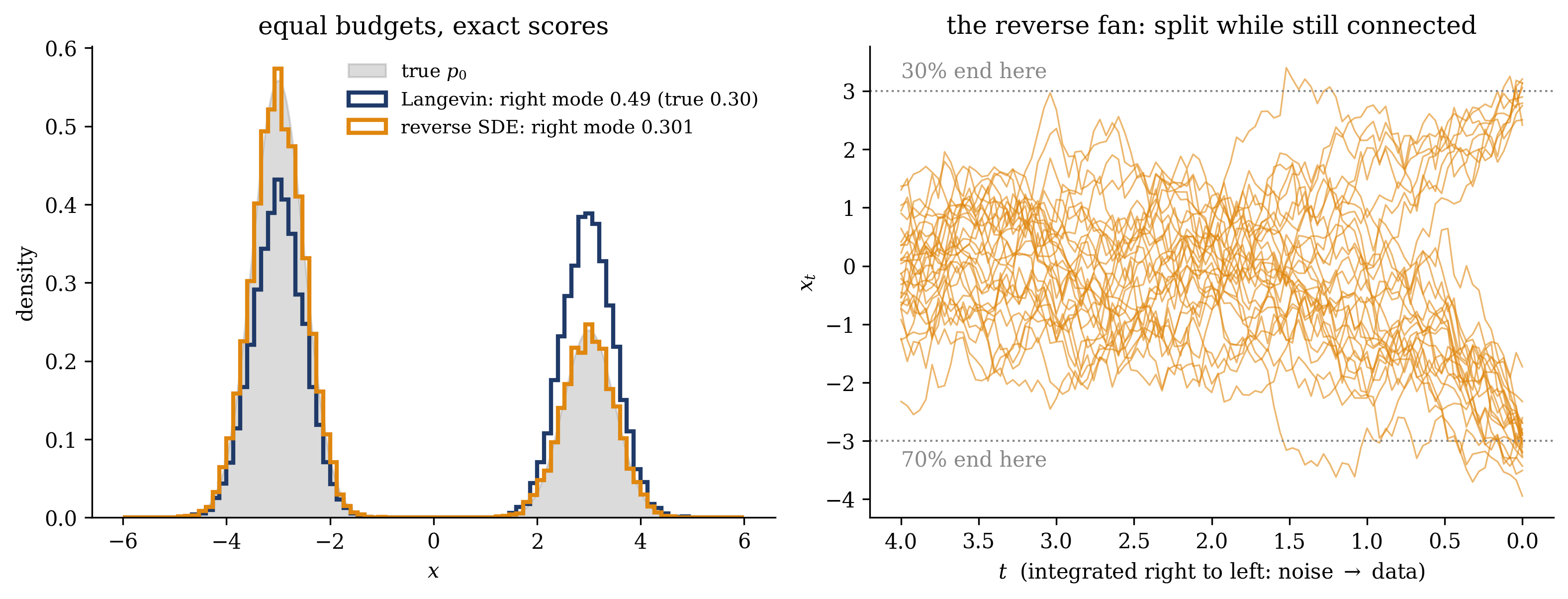
The result (Figure 20.3) is unambiguous. Langevin, with the true score in hand, reproduces two correctly shaped modes — carrying the wrong weights: \(0.49\) in the right-hand mode against a true \(0.30\). Its initialization split the particles roughly evenly between the two basins, and in 800 steps essentially no walker crossed the barrier; the sampler is locally perfect and globally frozen, exactly as Section 15.4 taught (and the histogram alone gives no warning). The reverse SDE, at the same cost, lands the mode weight at \(0.301\) — the truth to three decimals — because its particles never had to cross anything: they descended the filmstrip, splitting into the two modes in the correct proportions back when the modes were still connected blurs (the trajectory fan in the right panel shows the split happening around \(t \approx 1\), where Figure 20.2 shows the barrier only beginning to form). Mixing was not accelerated; it was made unnecessary.

Show code

rng = np.random.default_rng(0)
T, nsteps, npart = 4.0, 800, 20000
dt = T / nsteps

# transport: reverse-time SDE from noise, recording a fan of trajectories
x = rng.normal(0, 1, npart)
n_show, rec_every = 30, 8
fan = [x[:n_show].copy()]
for i in range(nsteps):
    t = T - i * dt
    drift = -x - 2 * score_t(x, t)                 # f - g^2 s, with f=-x, g^2=2
    x = x - drift * dt + np.sqrt(2 * dt) * rng.normal(size=npart)
    if (i + 1) % rec_every == 0:
        fan.append(x[:n_show].copy())
fan = np.array(fan)
w_rev = (x > 0).mean()

# equilibration: Langevin at t=0, same budget, same init
x2 = rng.normal(0, 1, npart)
for i in range(nsteps):
    x2 = x2 + score_t(x2, 0.0) * dt + np.sqrt(2 * dt) * rng.normal(size=npart)
w_lan = (x2 > 0).mean()

xs = np.linspace(-6, 6, 400)
fig, (a1, a2) = plt.subplots(1, 2, figsize=(10.6, 4.1))
a1.fill_between(xs, pt_density(xs, 0.0), color=GRAY, alpha=0.30, label="true $p_0$")
a1.hist(x2, bins=90, range=(-6, 6), density=True, histtype="step",
        color=NAVY, lw=2.0, label=rf"Langevin: right mode {w_lan:.2f} (true 0.30)")
a1.hist(x, bins=90, range=(-6, 6), density=True, histtype="step",
        color=ORANGE, lw=2.0, label=rf"reverse SDE: right mode {w_rev:.3f}")
a1.set_xlabel(r"$x$"); a1.set_ylabel("density")
a1.set_title("equal budgets, exact scores", fontsize=12)
a1.legend(frameon=False, fontsize=9)
ts_fan = T - rec_every * dt * np.arange(fan.shape[0])
for j in range(n_show):
    a2.plot(ts_fan, fan[:, j], color=ORANGE, lw=0.8, alpha=0.6)
a2.invert_xaxis()
a2.axhline(-3, color=GRAY, ls=":", lw=1); a2.axhline(3, color=GRAY, ls=":", lw=1)
a2.text(4.0, -3.15, "70% end here", color=GRAY, fontsize=10, va="top")
a2.text(4.0, 3.15, "30% end here", color=GRAY, fontsize=10, va="bottom")
a2.set_xlabel(r"$t$  (integrated right to left: noise $\to$ data)")
a2.set_ylabel(r"$x_t$")
a2.set_title("the reverse fan: split while still connected", fontsize=12)
fig.tight_layout(); plt.show()

Figure 20.3: Transport versus equilibration, with the exact score and identical budgets (800 steps, \(20{,}000\) particles, both started from \(\mathcal{N}(0,1)\)). Left: final samples against the true data density (gray). Plain Langevin at \(t=0\) (navy) produces perfectly shaped modes with frozen initialization weights — \(0.49\) in the right mode against a true \(0.30\): no barrier crossings in budget, and nothing in the histogram warns you. The reverse-time SDE Equation 20.2 (orange) lands the weight at \(0.301\). Right: a fan of reverse-SDE trajectories — read right to left, from noise at \(t = 4\) to data at \(t = 0\) — splitting into the two modes in the correct proportions while the marginals are still connected blurs (compare Figure 20.2). The barrier is never crossed because it is never encountered.

Generation is time reversal: corrupt the data to noise, learn the score of every intermediate blur, and run the film backwards — no \(Z\), and no waiting for mixing.

The tutorial (16–18, Ph12 106) is derivation-led, with two board problems. First, the reversal the warm-up card attempted — the one-dimensional Ornstein–Uhlenbeck process — done properly and by hand: with the general theorem now available, the exercise is to earn its simplest instance from scratch. Second, fit a two-dimensional score model by denoising score matching and generate from it. The tutorial also closes a connection left open since Week 3. The tutorial uses Equation 20.2 and Hyvärinen’s objective; no devices.

20.6 Outlook: the cost of running time backwards

Week 10 closes with the arc from statistical physics to generative modeling complete at the level of mathematics. The previous lecture removed the partition function from training: the score is blind to \(Z\), and Hyvärinen’s integration by parts made it learnable. Today removed equilibration from generation: Anderson’s theorem turns a fixed corruption process into an exact generative one, steered by the learned score, starting from the only distribution that requires no mixing. Between the two lectures, every obstruction this course has fought — the normalizer that blocked the Boltzmann machine, the mixing that priced every sampler — has been either dissolved or bypassed, and the machinery reduces to three components: a forward SDE, a regression loss, and a reverse SDE. The arc from Boltzmann to diffusion is, at this point, a theorem with a training procedure.

What remains of the module is physics — and it is the physics the module is named for. Running a distribution along a nonequilibrium path is not free: it dissipates, and next week the course meets the accounting identities that govern the cost. The Jarzynski equality and Crooks’ theorem relate the irreversible work of finite-time transports to equilibrium free-energy differences — nonequilibrium trajectories computing equilibrium quantities — and their machine-learning shadow, annealed importance sampling, resolves the open question from Module 3: extracting \(Z\) itself from chains that never equilibrate (the gap Section 15.4 conceded, now closed). And Week 12 assembles today’s pipeline into the industrial object — DDPM’s discrete steps and \(\varepsilon\)-parameterization, the probability-flow ODE, and the schedules.