19 Score matching: differentiating past the partition function

19.1 The partition function, revisited

Every module of this course has been shaped by the same object. Week 1 introduced the partition function \(Z = \sum_x e^{-E(x)}\) as the quantity that turns an energy into a probability, and flagged it as the recurring obstruction; Week 3 met the obstruction in earnest — the likelihood gradient of a Boltzmann machine needs \(\nabla_\theta \log Z\), the negative phase (Equation 5.5), an average over the model that no tractable computation supplies, and contrastive divergence survived only by dodging it and paying in bias (Section 6.4). Module 2 stopped fighting for \(\log Z\) exactly and bounded it, building the variational free energy (Equation 9.1) and everything through the VAE on that bound. Module 3 arranged for \(Z\) to cancel: the Metropolis rule needs only ratios (Section 15.3), and training itself turned out to be such a sampler. Each module found a different workaround — bounding, cancelling, dodging — but none eliminated \(Z\) from the equations.

The present lecture removes it. The partition function is an integral over all configurations: a number. It depends on the parameters \(\theta\) — hence Week 3’s obstruction — but it does not depend on which configuration \(x\) you happen to be looking at. To the configuration variable, \(Z\) is a constant, and constants have zero gradient:

\[ \nabla_x \log Z \;=\; 0 . \]

So the moment we differentiate \(\log p\) with respect to \(x\) rather than \(\theta\), the object that blocked energy-based learning disappears from the equations — eliminated not approximately but identically by the derivative. Hyvärinen (2005) built an estimation method on exactly this observation, score matching, which fits an unnormalized model to data with no \(Z\) anywhere; Vincent (2011) made it cheap (denoising); Song and Ermon (2019) turned it into state-of-the-art generation and set it on the road to diffusion. The idea is, in retrospect, straightforward: differentiate past the normalizer.

The question: how do you fit \(p = e^{-E}/Z\) to data when you cannot compute \(Z\)? First, fit the score \(\nabla_x \log p\) instead of the density — then \(Z\) drops out. Second, the remaining obstacle — that we do not know the score of the data either — falls to an integration by parts. What comes out is an exact, sampling-free objective for unnormalized models, and the object it estimates, the score, is precisely the drift a Langevin equation needs to generate.

Take-home 1

\(Z\) is a constant in \(x\), so \(\nabla_x \log Z = 0\): the score of an energy-based model is \(\nabla_x \log p = -\nabla_x E\), with no partition function anywhere. The obstruction that Week 1 named and Week 3 collided with is invisible to the configuration gradient — this is the resolution announced in the first lecture.

19.2 Two gradients of one constant

We state the escape as a dichotomy before using it, because the entire method is the choice between two derivatives of the same object. The parameter gradient \(\nabla_\theta \log Z = -\langle \nabla_\theta E \rangle_\text{model}\) is Week 3’s obstruction: not zero, not tractable, the negative phase that forced contrastive divergence. The configuration gradient \(\nabla_x \log Z\) is zero, identically, trivially. Same \(Z\); one derivative is the obstruction and the other does not exist. This is why every gradient in the course carries a subscript — the choice between \(\nabla_\theta\) and \(\nabla_x\) is what makes the removal visible. (The distinction appeared in Section 17.2 from the parameter-space side; the configuration-space counterpart is the present section.)

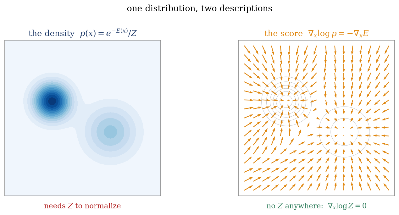
What does one gain by fitting \(\nabla_x \log p\) instead of \(p\)? Figure 19.1 shows the two descriptions of one and the same distribution. The density is a scalar field whose values must integrate to one — normalization is constitutive, and \(Z\) is its price. The score \(s(x) = \nabla_x \log p(x)\) is a vector field: at every point, an arrow pointing in the direction of increasing log-probability — toward the data, everywhere. Arrows carry no normalization; scaling \(p\) by any constant leaves every arrow untouched. And the arrows are not a lossy summary: up to the overall constant, the score determines the distribution (integrate it back up), and — the module’s coming theme — a field of arrows toward the data is already a generator, because it is exactly the drift that Week 9’s Langevin equation needs to sample \(p\).

Figure 19.1: The central picture of the lecture: one distribution, two descriptions. Left: the density \(p(x) = e^{-E(x)}/Z\) of a two-mode distribution — a scalar field that must integrate to one, which is what the partition function is for. Right: the score \(\nabla_x \log p = -\nabla_x E\) of the same distribution — a vector field of arrows pointing toward the data (gray contours: the density), invariant under any rescaling of \(p\), hence free of \(Z\). Score matching learns the right panel from samples; Langevin dynamics turns the right panel back into the left one.

A notational change: after serving as an Ising spin for six weeks, \(s\) now denotes the score — a gradient field over configuration space, ML’s standard symbol for it — and \(\sigma\) below is a noise scale, not a spin. The energy \(E(x)\) and its configuration gradient \(\nabla_x E\) are the objects of Weeks 1–3, unchanged.

19.3 The engine, part I: the score is \(Z\)-free

The first result is central, and the derivation is short. For an energy-based model \(p_\theta(x) = e^{-E_\theta(x)}/Z_\theta\),

\[ \boxed{\; s_\theta(x) \;=\; \nabla_x \log p_\theta(x) \;=\; \nabla_x \big( -E_\theta(x) - \log Z_\theta \big) \;=\; -\nabla_x E_\theta(x), \qquad \text{since } \nabla_x \log Z_\theta = 0 . \;} \tag{19.1}\]

the score is \(Z\)-free

The score of an unnormalized model is the negative gradient of its energy — computable, for any energy you can write down, by a single differentiation, with no knowledge of \(Z\) whatsoever. Contrast this with what Week 3 needed. Maximum likelihood differentiates \(\log p_\theta\) in \(\theta\), and there \(\log Z_\theta\) does not drop out: \(\nabla_\theta \log Z_\theta = -\langle \nabla_\theta E_\theta \rangle_\text{model}\), the negative phase, an expectation under the very distribution we cannot sample cheaply (Equation 5.5). The two statements sit side by side:

\[ \underbrace{\nabla_\theta \log Z_\theta = -\big\langle \nabla_\theta E_\theta \big\rangle_\text{model} \;\neq\; 0}_{\text{Week 3: the obstruction}} \qquad\qquad \underbrace{\nabla_x \log Z_\theta = 0}_{\text{today: the escape}} . \]

To be precise about what has and has not been achieved: \(Z_\theta\) is not made zero — it still exists, still depends on \(\theta\), and still cannot be computed. A different derivative of it is zero, and score matching is the estimation method that only ever needs that derivative. The remaining question is what to match the model score against. The natural target is the score of the data — which we do not know either, since we have samples from \(p_\text{data}\), not its formula. Removing that second unknown is Hyvärinen’s theorem.

19.4 The engine, part II: Hyvärinen’s theorem

The natural objective is to make the model’s score field match the data’s, in mean square under the data distribution — the Fisher divergence:

\[ J(\theta) \;=\; \frac{1}{2}\, \Big\langle \big\| s_\theta(x) - \nabla_x \log p_\text{data}(x) \big\|^2 \Big\rangle_{p_\text{data}} , \]

which vanishes exactly when \(s_\theta\) equals the data score (almost everywhere), so its minimizer recovers the true model when the family contains it (Hyvärinen 2005). As written it is useless: it contains \(\nabla_x \log p_\text{data}\), the score of an unknown density. Expand the square and note where the unknown sits,

\[ J(\theta) \;=\; \Big\langle \tfrac{1}{2} \|s_\theta\|^2 \Big\rangle_{p_\text{data}} - \Big\langle s_\theta \cdot \nabla_x \log p_\text{data} \Big\rangle_{p_\text{data}} + \underbrace{\Big\langle \tfrac{1}{2} \|\nabla_x \log p_\text{data}\|^2 \Big\rangle_{p_\text{data}}}_{\text{independent of } \theta} : \]

the first term is pure model, the last is a constant we may discard, and only the cross term couples to the unknown. That term is the target of the next manipulation. Write the expectation as an integral and use \(p_\text{data} \nabla_x \log p_\text{data} = \nabla_x p_\text{data}\):

\[ - \Big\langle s_\theta \cdot \nabla_x \log p_\text{data} \Big\rangle_{p_\text{data}} \;=\; - \int \mathrm{d}x \; s_\theta(x) \cdot \nabla_x p_\text{data}(x) \;=\; + \int \mathrm{d}x \; p_\text{data}(x) \, \nabla_x \cdot s_\theta(x), \]

integrating by parts in each coordinate, with the boundary terms vanishing provided \(p_\text{data}(x)\, s_\theta(x) \to 0\) at infinity (true for any decaying density and reasonable model; the regularity assumptions are stated in full in Hyvärinen (2005), and they can genuinely fail on bounded domains or heavy tails — this is the theorem’s fine print). The unknown data score is gone: differentiation has been thrown from the data onto the model, where we can afford it. Reassembling,

\[ \boxed{\; J(\theta) \;=\; \Big\langle \tfrac{1}{2}\, \|s_\theta(x)\|^2 \;+\; \operatorname{tr} \nabla_x s_\theta(x) \Big\rangle_{p_\text{data}} \;+\; \text{const}, \;} \tag{19.2}\]

Hyvärinen’s score-matching objective

an expectation over the data of two quantities computable at any sample point: the squared norm of the model score, and its divergence \(\operatorname{tr} \nabla_x s_\theta = \sum_i \partial^2 \log p_\theta / \partial x_i^2\). For an energy-based model, using Equation 19.1, the objective reads

\[ J(\theta) \;=\; \Big\langle \tfrac{1}{2}\, \|\nabla_x E_\theta\|^2 \;-\; \nabla_x^2 E_\theta \Big\rangle_{p_\text{data}} + \text{const} : \tag{19.3}\]

score matching for an EBM

the mean squared force minus the mean Laplacian of the energy, evaluated on data points. The intractability of energy-based learning has been transformed: the negative phase — an average over the model, requiring sampling — has been replaced entirely by averages over the data, requiring nothing but derivatives of the energy at points you already have. There is no \(Z\), no Monte Carlo, and no bias. The two removals compose: \(\nabla_x \log Z = 0\) deleted the normalizer, and integration by parts deleted the data score. What maximum likelihood could not do exactly for a single unnormalized model, score matching does exactly for all of them.

The price is a change of divergence: score matching minimizes the Fisher divergence, not the KL divergence of maximum likelihood. The estimator is consistent — with a realizable model and enough data it recovers the same truth — but at finite samples the two weight errors differently (Fisher divergence is comparatively insensitive to getting the mixture weights of well-separated modes right, precisely because so little data sits between the modes). It is a different estimator, not a reparameterized likelihood.

Take-home 2

Integration by parts moves the derivative off the unknown data score and onto the model: the Fisher divergence becomes Hyvärinen’s objective \(J = \langle \frac{1}{2}\|s_\theta\|^2 + \operatorname{tr} \nabla_x s_\theta \rangle_{p_\text{data}} + \text{const}\) (Equation 19.2), computable from samples alone under mild boundary assumptions. Together with \(\nabla_x \log Z = 0\), an unnormalized model is fitted exactly with no partition function and no sampling — at the price of minimizing the Fisher divergence rather than the KL.

19.5 What score matching delivers, and the road to diffusion

The deliverable is a score, not a density. Score matching estimates \(-\nabla_x E\), equivalently the energy up to an additive constant — and that constant is exactly \(\log Z\), which the method neither recovers nor needs. You cannot evaluate \(p_\theta(x)\); you cannot compare likelihoods. What you can do is generate: the score is the drift of the configuration-space Langevin equation

\[ \mathrm{d}x \;=\; s_\theta(x)\, \mathrm{d}t + \sqrt{2}\, \mathrm{d}W, \]

whose stationary distribution is \(p_\theta\) — Week 9’s machinery (Equation 17.3) transplanted from parameters to data, with the learned arrows of Figure 19.1 doing the steering. A fitted score field is a working sampler of an unnormalizable model. This structural fact is the module’s foundation: generation needs the score, not the density, and the score carries no normalizer.

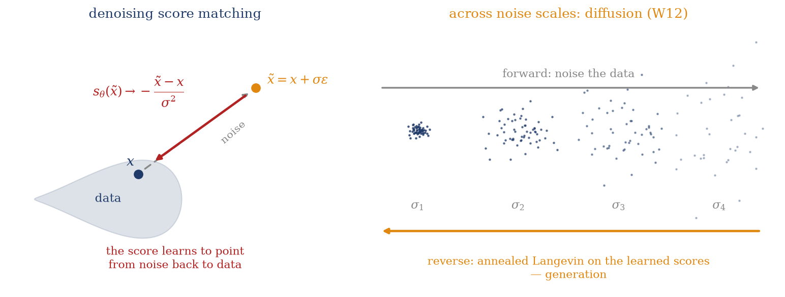
The cost, and the denoising fix. The divergence term in Equation 19.2 is the objection in high dimension: \(\operatorname{tr} \nabla_x s_\theta\) is a Jacobian trace, costing on the order of \(d\) backpropagations per data point. Vincent (2011) removed it with a move that looks like a compromise and proved decisive. Perturb each data point with Gaussian noise, \(\tilde{x} = x + \sigma \varepsilon\), \(\varepsilon \sim \mathcal{N}(0, I)\), and match the score of the noised distribution \(q_\sigma\). The conditional score is closed-form, \(\nabla_{\tilde{x}} \log q_\sigma(\tilde{x} \mid x) = -(\tilde{x} - x)/\sigma^2\), and Vincent’s identity states that regressing on it is equivalent (up to a \(\theta\)-independent constant) to score-matching the noised marginal:

\[ J_\text{DSM}(\theta) \;=\; \frac{1}{2}\, \Big\langle \big\| s_\theta(\tilde{x}) + \frac{\tilde{x} - x}{\sigma^2} \big\|^2 \Big\rangle_{x \sim p_\text{data},\; \tilde{x} \sim q_\sigma(\cdot \mid x)} , \tag{19.4}\]

denoising score matching

with minimizer \(s_\theta = \nabla \log q_\sigma\), the score of the data smoothed at scale \(\sigma\). (The identity is two lines: expanding the square, the cross term \(\langle s_\theta \cdot \nabla_{\tilde x} \log q_\sigma(\tilde x \mid x)\rangle\) collapses by \(\int \mathrm{d}x\, p_\text{data}(x)\, q_\sigma(\tilde x \mid x) \nabla_{\tilde x} \log q_\sigma(\tilde x \mid x) = \nabla_{\tilde x} q_\sigma(\tilde x)\) into the same cross term with the marginal’s score — no integration by parts, no Jacobian.) The objective is a task: the model is handed a noised point and trained to predict the direction back to the clean one — denoising. Matching scores and removing noise are the same problem (Figure 19.2, left). Sliced score matching (Song et al. 2020), which estimates the Jacobian trace with random projections, is the other scalable route; denoising is the one history chose.

The bridge to Week 12. A score learned at one small noise scale inherits a weakness of Langevin sampling itself: in the low-density regions between modes there is almost no data, the learned arrows are unreliable there (the example below catches this happening), and a sampler must cross exactly those regions to mix. The repair of Song and Ermon (2019) is to learn the score at many noise scales — heavily smoothed distributions have no empty regions — and generate by annealed Langevin: start from pure noise where the coarse score is trustworthy, and step down the noise ladder as the samples approach the data (Figure 19.2, right). Forward noising, a learned family of denoising scores, a reverse pass from noise to data: this is a diffusion model in everything but name, and the per-scale training loss is Equation 19.4. The next lecture supplies the missing mathematics — Anderson’s reverse-time SDE, which makes “run the noising backwards” an exact equation with the score as its only unknown — and Week 12 assembles the full machine. The object everything runs on is the \(Z\)-free score built today.

Figure 19.2: Denoising score matching, and where it leads. Left: a data point \(x\) is perturbed to \(\tilde{x} = x + \sigma\varepsilon\) (gray dashed), and the score model is trained to point back, \(s_\theta(\tilde{x}) \to -(\tilde{x} - x)/\sigma^2\) (red): matching the score of noised data is denoising — no Jacobian trace, no partition function. Right: the same idea across a ladder of noise scales \(\sigma_1 < \dots < \sigma_4\): the forward direction noises data into a featureless cloud; generation runs the ladder in reverse by annealed Langevin on the learned scores (Song and Ermon 2019). This is a diffusion model in embryo, trained per scale by Equation 19.4 — Week 12’s subject.

Trap

Three standard errors. ① The escape is \(\nabla_x \log Z = 0\) — the configuration gradient. Week 3’s obstruction \(\nabla_\theta \log Z\), the parameter gradient, is not zero and never became zero; a different derivative of the same object vanishes. Conflating the two subscripts erases the entire logic of the course’s spine. ② Score matching delivers an unnormalized model: the energy up to an additive constant (\(= \log Z\)), a sampler (via Langevin), but never \(p_\theta(x)\) or a likelihood. ③ Hyvärinen’s integration by parts has fine print — boundary terms must vanish and the Fisher divergence is not the KL — so the exactness claim is “exact under stated assumptions, for a different divergence,” not “maximum likelihood for free.”

Take-home 3

Score matching yields the score (the energy up to the constant \(\log Z\)): you can sample it by Langevin — the score is the drift, Week 9’s machinery in configuration space — but not evaluate the density. The Jacobian-trace cost is removed by denoising score matching (Equation 19.4): match the score of noise-perturbed data, which is a denoising task, and exactly a diffusion model’s per-scale training loss. Learned across noise scales with annealed Langevin (Song and Ermon 2019), the \(Z\)-free score becomes a generator — Week 12 in embryo.

19.6 Example: a model fitted with no \(Z\)

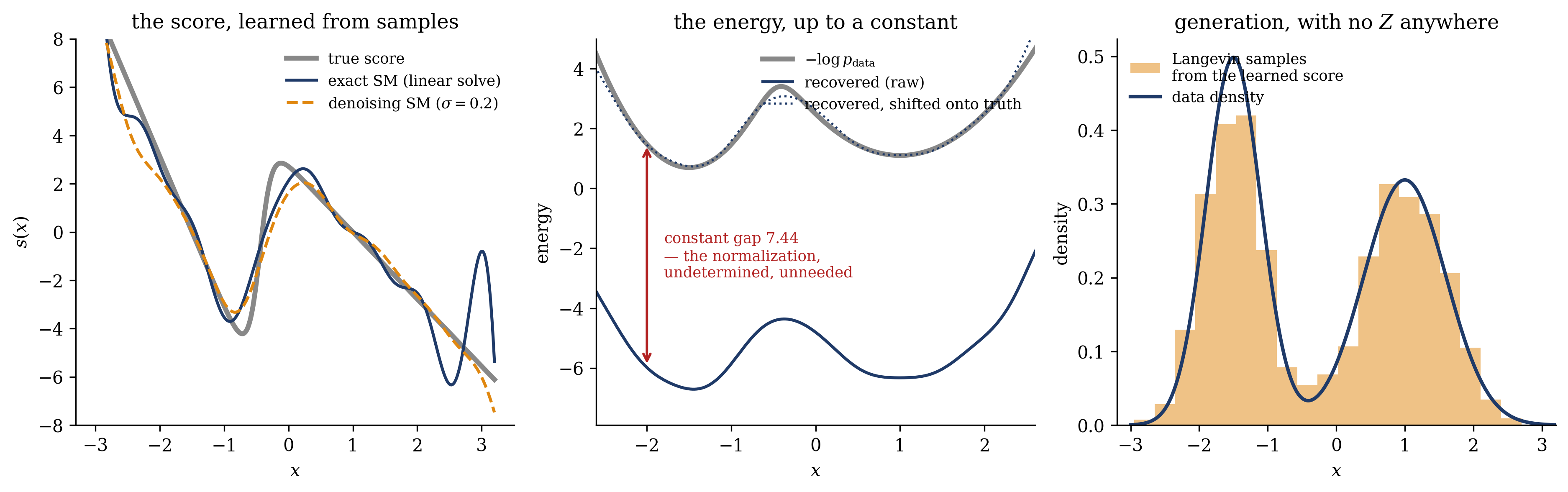
We now make the removal operational on the smallest nontrivial case, with an additional simplification: for a score model linear in its parameters, \(s_\theta(x) = \sum_k w_k \varphi_k(x)\) with fixed basis functions \(\varphi_k\), Hyvärinen’s objective Equation 19.2 is quadratic in \(w\), so exact score matching reduces to solving a linear system — no gradient descent and no neural network, the estimator in its purest form. Take \(5000\) samples from a two-mode Gaussian mixture, a basis of \(25\) Gaussian bumps, and fit three ways of looking at the same estimate (Figure 19.3).

The left panel is the estimator at work: the fitted score (navy) tracks the true mixture score (gray) closely wherever data lives, and denoising score matching at \(\sigma = 0.2\) (orange dashed) recovers essentially the same field — from noised samples, with no divergence term. Both fits wobble beyond \(|x| \gtrsim 2.5\), and the wobble is expected: score matching weights its objective by \(p_\text{data}\), so the score is simply unconstrained where the data does not go — the low-density blind spot that multi-scale noise (Week 12) exists to fix. The middle panel illustrates the central point: integrating the fitted score gives the energy, and the recovered curve runs parallel to the true \(-\log p\) — the vertical gap between them is constant to within \(0.11\) across the data region. An additive constant is exactly what a gradient cannot see, and for \(p = e^{-E}/Z\) the normalization \(\log Z\) lives in that constant: the one object score matching cannot deliver is the one it was built to avoid. The right panel closes the loop: Langevin sampling with the learned score as drift regenerates the data density, placing \(49.1\%\) of its samples in the left mode against the true \(50\%\) — generation from a model whose normalizer was never computed.

Show code

rng = np.random.default_rng(10)

# data: two-component Gaussian mixture
w1, m1, sd1 = 0.5, -1.5, 0.4
w2, m2, sd2 = 0.5, 1.0, 0.6
n = 5000
comp = rng.random(n) < w2
x = np.where(comp, m2 + sd2 * rng.standard_normal(n),
             m1 + sd1 * rng.standard_normal(n))

def pdf(t):
    g1 = np.exp(-(t - m1) ** 2 / (2 * sd1**2)) / (sd1 * np.sqrt(2 * np.pi))
    g2 = np.exp(-(t - m2) ** 2 / (2 * sd2**2)) / (sd2 * np.sqrt(2 * np.pi))
    return w1 * g1 + w2 * g2

def true_score(t, eps=1e-4):
    return (np.log(pdf(t + eps)) - np.log(pdf(t - eps))) / (2 * eps)

# linear-in-parameters score model: s(x) = sum_k w_k phi_k(x), Gaussian bumps
K, h = 25, 0.5
c = np.linspace(-4.0, 4.0, K)
phi = lambda t: np.exp(-(t[:, None] - c[None, :]) ** 2 / (2 * h**2))
dphi = lambda t: -(t[:, None] - c[None, :]) / h**2 * phi(t)

# exact Hyvarinen SM: J = 1/2 w^T E[phi phi^T] w + E[phi']^T w  ->  linear solve
P = phi(x)
A = P.T @ P / n
b = dphi(x).mean(axis=0)
w_sm = -np.linalg.solve(A + 1e-6 * np.eye(K), b)

# denoising SM at scale sigma: least squares onto the target -eps/sigma
sig = 0.2
eps = rng.standard_normal(n)
xt = x + sig * eps
Pt = phi(xt)
w_dsm = -np.linalg.solve(Pt.T @ Pt / n + 1e-6 * np.eye(K),
                         Pt.T @ (eps / sig) / n)

tt = np.linspace(-3.0, 3.2, 500)
s_sm, s_dsm = phi(tt) @ w_sm, phi(tt) @ w_dsm

# energy recovery: E = -integral of s, defined up to a constant
dt = tt[1] - tt[0]
E_rec = -np.cumsum(s_sm) * dt
E_true = -np.log(pdf(tt))
mask = (tt > -2.4) & (tt < 2.4)
off = (E_true - E_rec)[mask].mean()

# Langevin sampling from the learned score
nw, ns, step = 4000, 3000, 5e-3
xs = 2.0 * rng.standard_normal(nw)
for _ in range(ns):
    xs = xs + step * (phi(xs) @ w_sm) + np.sqrt(2 * step) * rng.standard_normal(nw)

fig, (a1, a2, a3) = plt.subplots(1, 3, figsize=(12.6, 4.0))
a1.plot(tt, true_score(tt), color=GRAY, lw=2.8, label="true score")
a1.plot(tt, s_sm, color=NAVY, lw=1.7, label="exact SM (linear solve)")
a1.plot(tt, s_dsm, color=ORANGE, lw=1.7, ls="--",
        label=rf"denoising SM ($\sigma = {sig}$)")
a1.set_ylim(-8, 8)
a1.set_xlabel(r"$x$"); a1.set_ylabel(r"$s(x)$")
a1.set_title("the score, learned from samples", fontsize=11.5)
a1.legend(frameon=False, fontsize=8.5, loc="upper right")

a2.plot(tt, E_true, color=GRAY, lw=2.8, label=r"$-\log p_\mathrm{data}$")
a2.plot(tt, E_rec, color=NAVY, lw=1.7, label="recovered (raw)")
a2.plot(tt, E_rec + off, color=NAVY, lw=1.2, ls=":",
        label="recovered, shifted onto truth")
i2 = np.argmin(np.abs(tt + 2.0))
a2.annotate("", xy=(-2.0, E_true[i2]), xytext=(-2.0, E_rec[i2]),
            arrowprops=dict(arrowstyle="<->", color=RED, lw=1.4))
a2.text(-1.8, (E_true[i2] + E_rec[i2]) / 2,
        f"constant gap ${off:.2f}$\n— the normalization,\nundetermined, unneeded",
        fontsize=8.5, color=RED, va="center")
a2.set_xlim(-2.6, 2.6)
a2.set_ylim(E_rec[mask].min() - 1.2, E_true[mask].max() + 1.2)
a2.set_xlabel(r"$x$"); a2.set_ylabel(r"energy")
a2.set_title("the energy, up to a constant", fontsize=11.5)
a2.legend(frameon=False, fontsize=8.5, loc="upper right")

a3.hist(xs, bins=80, density=True, color=ORANGE, alpha=0.5,
        label="Langevin samples\nfrom the learned score")
a3.plot(tt, pdf(tt), color=NAVY, lw=2.0, label="data density")
a3.set_xlim(-3.2, 3.2)
a3.set_xlabel(r"$x$"); a3.set_ylabel("density")
a3.set_title("generation, with no $Z$ anywhere", fontsize=11.5)
a3.legend(frameon=False, fontsize=8.5, loc="upper left")
fig.tight_layout(); plt.show()

Figure 19.3: Score matching with no partition function, on \(5000\) samples from the mixture \(\frac{1}{2}\mathcal{N}(-1.5, 0.4^2) + \frac{1}{2}\mathcal{N}(1.0, 0.6^2)\), using a score model linear in \(25\) Gaussian basis functions (Hyvärinen’s objective is then quadratic — solved exactly by linear algebra). Left: the fitted score (navy) against the true mixture score (gray); denoising score matching at \(\sigma = 0.2\) (orange dashed) recovers the same field from noised samples with no divergence term. Both wobble outside the data region (\(|x| \gtrsim 2.5\)) — score matching is data-weighted, and the score is unconstrained where the density vanishes: the blind spot that motivates multiple noise scales (W12). Middle: integrating the fitted score recovers the energy up to an additive constant — the raw recovered curve (navy) runs parallel to the true \(-\log p\) (gray), their gap constant to within \(0.11\) across the data region; that gap (the integration constant, where \(\log Z\) hides) is exactly the information score matching discards. Right: Langevin sampling with the learned score as drift regenerates the data density, with \(49.1\%\) of samples in the left mode against the true \(50\%\) — generation from a never-normalized model.

19.7 Outlook: the spine, resolved

The next lecture takes the reverse-time SDE up in full generality (Anderson’s 1982 result): a learned score is not merely a Langevin drift but the exact ingredient that inverts any diffusion — the mathematical heart of Week 12’s generative models. The tutorial (Ph12 106) is derivation-led: you will fit a two-dimensional score model with Hyvärinen’s objective, and derive by hand — for the one-dimensional Ornstein–Uhlenbeck process you now know well — the reverse-time SDE that turns a forward noising process into a generator. The tutorial connects Equation 19.2 to Week 3’s RBM fitting: the object that blocked training there has a specific relationship to today’s score, and the session’s concluding exercise makes the connection explicit.

The wider map of the module: Week 11 turns nonequilibrium thermodynamics itself into an estimator — the Jarzynski and Crooks fluctuation theorems (Jarzynski 1997; Crooks 1999) extract equilibrium free-energy differences from driven trajectories, annealed importance sampling being their ML incarnation — and Week 12 assembles diffusion models (DDPM, score-SDE (Ho, Jain, and Abbeel 2020; Song et al. 2021)) from the parts now on the table: a forward noising process (Week 9’s Fokker–Planck), a score learned by denoising (Equation 19.4), and a reverse-time equation (the next lecture). Every ingredient of a diffusion model is now in place.

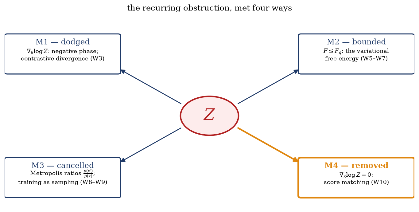
Figure 19.4 summarizes the course’s four encounters with \(Z\). The partition function was met four ways across four modules: dodged by contrastive divergence, which traded exactness for tractability; bounded by the variational free energy, which traded tightness for a guarantee; cancelled by Metropolis ratios, which traded closed forms for samples; and now removed by the configuration gradient, which traded the density for the score — and found that generation does not need the density in the first place.

Figure 19.4: The course’s spine, closed. The partition function \(Z\) — the recurring obstruction named in Week 1 — was met four ways across four modules: dodged (Module 1: the negative phase \(\nabla_\theta \log Z\) forced contrastive divergence), bounded (Module 2: the variational free energy \(F \leq F_q\)), cancelled (Module 3: Metropolis ratios, training as sampling), and finally removed (Module 4: \(\nabla_x \log Z = 0\), score matching). Each escape paid a different price; the last one pays with the normalization itself, which generative modeling turns out not to need.

The partition function is a constant to the score — and constants have zero gradient.