10 The mean-field ferromagnet: order from an approximation

10.1 The ferromagnet

The previous lecture built the variational machinery; today we apply it to the ferromagnet. The central equation: minimize the variational free energy over factorized distributions and each spin settles into the average field of its neighbors, \(m_i = \tanh\big(\beta(\sum_j J_{ij} m_j + h_i)\big)\) — an equation that is simultaneously Weiss’s molecular field and coordinate-ascent variational inference. (The equation always admits \(m = 0\) — the question is when it also admits nonzero solutions.)

Applied to the simplest interacting system — a ferromagnet, every spin nudging its neighbors toward alignment — a phase transition falls out. Below a sharp critical temperature, a second solution appears, the symmetric one destabilizes, and the system magnetizes spontaneously: collective order, predicted by an approximation that treats every spin as independent. Historically, this is where the subject’s language was established: Curie (1895) measured the ferromagnetic transition and the susceptibility law that bears his name; Weiss (1907) explained both with the molecular field — the previous lecture’s equation, applied and solved; and Landau (1937) abstracted the phenomenon into the universal vocabulary — order parameter, symmetry breaking, a free energy expanded in powers of the order — that physics now applies to every transition it meets, including, this course keeps finding, the ones inside learning machines (Week 2’s memory collapse already spoke this language; today we learn it properly).

The same equation, applied to a one-dimensional chain, predicts a transition at \(T_c = 2J\) — and there is no transition in one dimension at all. The true 1D Ising model orders only at \(T = 0\); the mean-field prediction is qualitatively wrong — a clean calculation that produces order where none exists. The lecture therefore has two halves: the transition itself, and the audit of when to trust the approximation that predicts it.

Take-home 1

Applied to the ferromagnet, the mean-field equation produces a phase transition: below \(T_c\) the system spontaneously magnetizes — collective order from an approximation. But the same approximation misplaces the order it predicts: wrong \(T_c\), spurious transitions in low dimension. The lecture presents the transition and then audits its validity.

10.2 The transition

Setup. Make the system homogeneous so one number carries everything: every site couples ferromagnetically to its neighbors, and by symmetry every site has the same magnetization, \(m_i = m\). Write \(J_0 \equiv \sum_j J_{ij}\) for the total coupling a site feels: for a lattice of coordination \(z\) with bonds \(J\), \(J_0 = zJ\); for the fully-connected normalization \(J_{ij} = J/N\) of the previous lecture’s example, \(J_0 = J(N-1)/N \to J\). (A symbol caution: the previous lecture used \(J_0\) for the coupling amplitude in \(J_{ij} = J_0/N\); here it is the summed field \(\sum_j J_{ij}\) — the two agree as \(N \to \infty\) but differ by \((N-1)/N\) at finite \(N\).) At zero external field, the previous lecture’s equations collapse to a single scalar self-consistency:

\[ m \;=\; \tanh(\beta J_0\, m). \]

We now face that question head-on: \(m = 0\) solves this at every temperature. When does anything else?

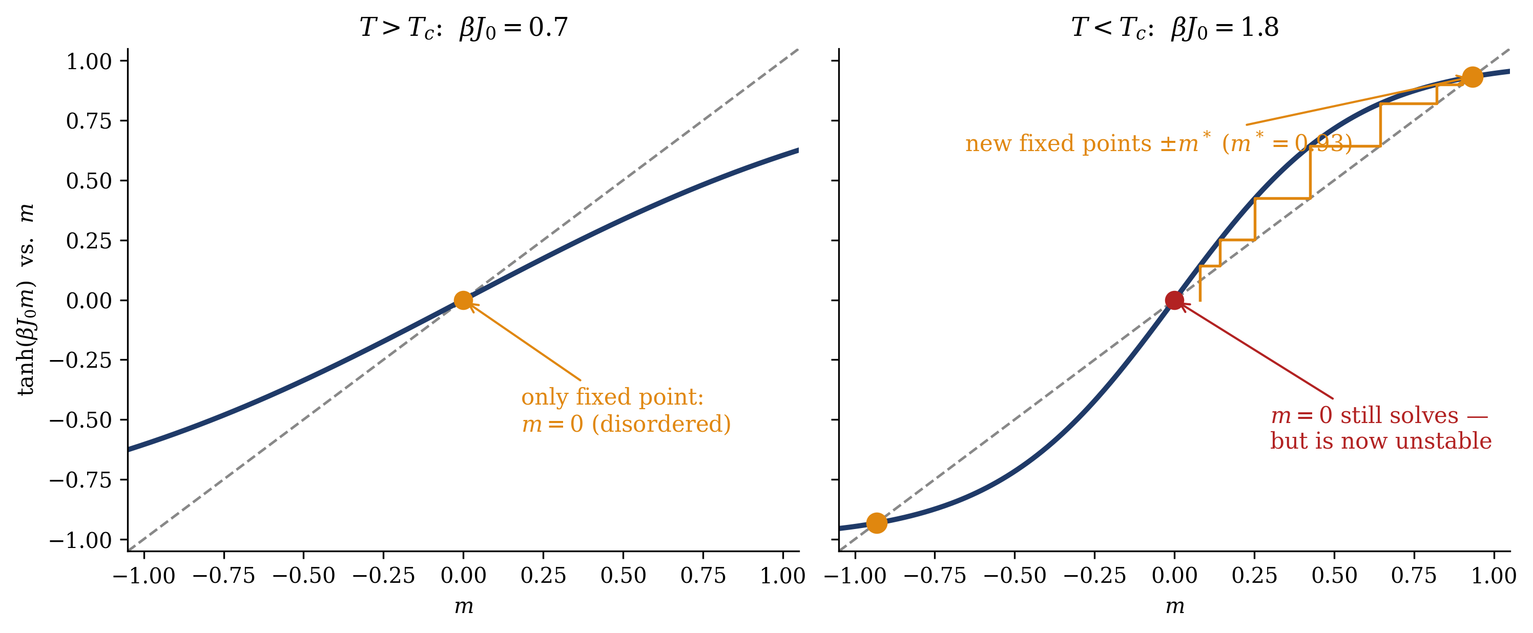
The graphical solution. Plot both sides (Figure 10.1): the diagonal \(y = m\) and the curve \(y = \tanh(\beta J_0 m)\). Both pass through the origin, so everything hinges on which is steeper there — the \(\tanh\) leaves the origin with slope \(\beta J_0\). If \(\beta J_0 \leq 1\), the \(\tanh\) starts below the diagonal and stays below: the origin is the only intersection, and the system is disordered. If \(\beta J_0 > 1\), the \(\tanh\) starts steeper than the diagonal, rises above it, and — being bounded — must bend back and recross it: two new intersections \(\pm m^*\) appear, symmetric about the origin. The threshold is exact and immediate:

\[ \beta_c\, J_0 = 1, \qquad\text{i.e.}\qquad T_c = J_0 \tag{10.1}\]

mean-field critical temperature

Physically: order sets in when the thermal energy drops below the total coupling a spin feels. For coordination \(z\) this reads \(T_c = zJ\): more neighbors, higher transition temperature — a first quiet hint of the validity story to come, since “more neighbors” is also what makes the mean field a better approximation.

Show code

fig, axes = plt.subplots(1, 2, figsize=(10.2, 4.2), sharey=True)
mm = np.linspace(-1.05, 1.05, 400)
for ax, bJ, ttl in zip(axes, [0.7, 1.8],
                       [r"$T > T_c$:  $\beta J_0 = 0.7$", r"$T < T_c$:  $\beta J_0 = 1.8$"]):
    ax.plot(mm, mm, color=GRAY, ls="--", lw=1.2)
    ax.plot(mm, np.tanh(bJ * mm), color=NAVY, lw=2.4)
    ax.plot([0], [0], "o", color=(ORANGE if bJ < 1 else RED), ms=8, zorder=4)
    ax.set_title(ttl, fontsize=12)
    ax.set_xlabel(r"$m$")
    ax.set_xlim(-1.05, 1.05); ax.set_ylim(-1.05, 1.05)
axes[0].set_ylabel(r"$\tanh(\beta J_0 m)$  vs.  $m$")
axes[0].annotate("only fixed point:\n$m=0$ (disordered)", xy=(0, 0), xytext=(0.18, -0.55),
                 color=ORANGE, fontsize=10.5,
                 arrowprops=dict(arrowstyle="->", color=ORANGE, lw=1))
# cobweb on the ordered side
bJ = 1.8
mstar = 0.99
for _ in range(200):
    mstar = np.tanh(bJ * mstar)
x = 0.08
xs, ys = [x], [0.0]
for _ in range(8):
    y = np.tanh(bJ * x); xs += [x, y]; ys += [y, y]; x = y
axes[1].plot(xs, ys, color=ORANGE, lw=1.3)
axes[1].plot([mstar, -mstar], [mstar, -mstar], "o", color=ORANGE, ms=9, zorder=4)
axes[1].annotate(rf"new fixed points $\pm m^*$ ($m^*={mstar:.2f}$)",
                 xy=(mstar, mstar), xytext=(-0.05, 0.62), ha="center",
                 color=ORANGE, fontsize=10.5,
                 arrowprops=dict(arrowstyle="->", color=ORANGE, lw=1))
axes[1].annotate("$m=0$ still solves —\nbut is now unstable", xy=(0, 0),
                 xytext=(0.3, -0.62), color=RED, fontsize=10.5,
                 arrowprops=dict(arrowstyle="->", color=RED, lw=1))
fig.tight_layout(); plt.show()

Figure 10.1: The graphical solution of \(m = \tanh(\beta J_0 m)\), the engine’s first picture. Left, \(T > T_c\) (drawn at \(\beta J_0 = 0.7\)): the \(\tanh\) leaves the origin with slope \(\beta J_0 < 1\), stays below the diagonal, and the only fixed point is \(m = 0\) — disorder. Right, \(T < T_c\) (\(\beta J_0 = 1.8\)): the origin slope exceeds one, the curve rises above the diagonal and bends back, and two new fixed points \(\pm m^*\) appear (here \(m^* = 0.93\)); the cobweb shows the previous lecture’s coordinate-ascent iteration \(m \leftarrow \tanh(\beta J_0 m)\) flowing away from the now-unstable origin and into the ordered solution. The transition is the moment the origin slope crosses one: \(T_c = J_0\).

Below \(T_c\), then, three solutions coexist: \(0\) and \(\pm m^*\). Which does the system take? The cobweb in the figure already suggests the answer — the previous lecture’s fixed-point iteration flows away from the origin and into \(\pm m^*\) — but “the iteration goes there” is dynamics, not thermodynamics. The previous lecture’s variational principle provides the answer: among multiple self-consistent solutions, take the one of lowest variational free energy. So we must now look at \(F_q\) itself — and looking at it is the second half of the engine, because the transition turns out to be a change in the shape of a landscape.

10.3 Landau’s landscape

The free energy as a function of the order parameter. For the homogeneous ansatz, the previous lecture’s variational free energy per spin is a function of the single number \(m\):

\[ f(m) \;=\; \frac{\langle E \rangle_q}{N} - T\, s(m) \;=\; -\tfrac{1}{2} J_0\, m^2 \;-\; T\, s(m), \]

with the binary entropy \(s(m)\) of Section 9.5 (the \(\tfrac12\) is the shared-bond bookkeeping, as in the previous lecture: \(\langle E\rangle_q = -\tfrac12 \sum_{i\neq j} J_{ij} m^2 = -\tfrac{N}{2} J_0 m^2\)). You have met this exact function before, in a different context: it is the \(f(m) = \varepsilon(m) - T s(m)\) whose saddle Section 2.5 evaluated for the all-to-all ferromagnet, back when it was a Week 1 exercise in Laplace’s method. That recognition returns below.

Expand near the transition. Everything near \(T_c\) happens at small \(m\), so expand. The entropy’s Taylor series follows from \(\partial S/\partial m = -\operatorname{artanh}(m) = -(m + m^3/3 + \cdots)\):

\[ s(m) \;=\; \log 2 \;-\; \frac{m^2}{2} \;-\; \frac{m^4}{12} \;-\; \cdots \]

and assembling \(f\):

\[ \boxed{\; f(m) \;\approx\; -T\log 2 \;+\; \frac{T - T_c}{2}\, m^2 \;+\; \frac{T}{12}\, m^4 \;+\; \cdots \;} \tag{10.2}\]

Landau free energy

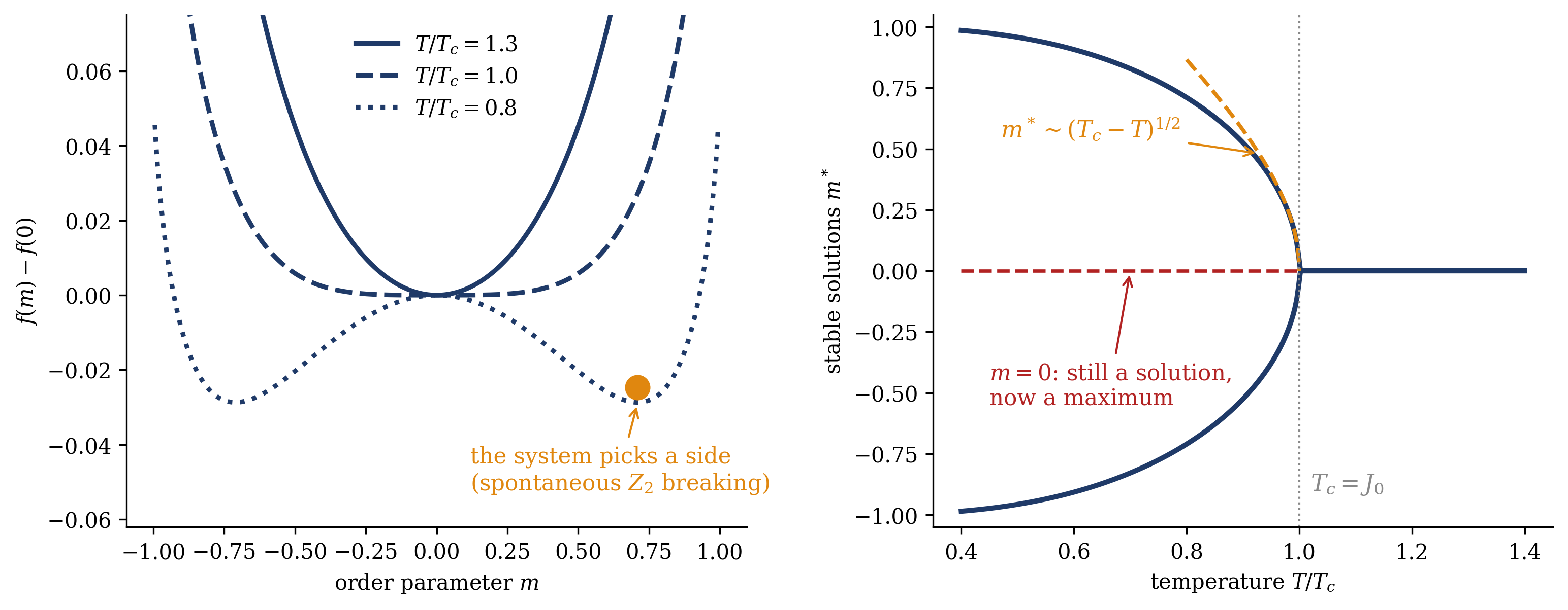
This is the Landau free energy, and its entire content sits in the quadratic coefficient \(a(T) = (T - T_c)/2\), which changes sign at \(T_c\) — the same \(T_c = J_0\) as the graphical argument, reassuringly. For \(T > T_c\): a single well at \(m = 0\); disorder is the minimum. For \(T < T_c\): the origin curves downward — the symmetric solution still exists but is now a local maximum — and the positive quartic term (\(b = T/12 > 0\)) catches the landscape on both sides, creating two symmetric minima at \(\pm m^*\). Figure 10.2 draws the morphing landscape and the pitchfork of solutions it implies. The transition is a change in the shape of a landscape, with temperature as the control parameter — the same picture as Figure 3.1, now derived from a variational principle.

Spontaneous symmetry breaking. Look at what has happened to the symmetry. The Hamiltonian at \(h = 0\) is exactly invariant under the global flip \(s \to -s\), so \(f(m) = f(-m)\): the law is \(Z_2\)-symmetric at every temperature. But below \(T_c\) the state is not: the system sits in one well, \(+m^*\) or \(-m^*\), and which one is decided by an infinitesimal stray field or the memory of history. The symmetry of the law is not the symmetry of the solution — spontaneous symmetry breaking, the concept Landau (1937) built the modern theory of phases around. One caveat, kept precise in the script: at finite \(N\) the system tunnels between the two wells and the literal average \(\langle m \rangle\) vanishes; broken symmetry is a statement about noncommuting limits (\(h \to 0\) after \(N \to \infty\)), i.e. about ergodicity breaking — the barrier between the wells becomes extensive and the two ordered states become separate worlds. Week 2’s stored memories were exactly such separate worlds; the vocabulary is the same because the phenomenon is.

The critical exponent. How fast does order grow below the transition? Minimize Equation 10.2: \(0 = (T - T_c)\,m + \tfrac{T}{3} m^3\) gives

\[ m^{*2} = \frac{3\,(T_c - T)}{T} \qquad\Longrightarrow\qquad \boxed{\; m^* \;\sim\; (T_c - T)^{1/2} \;} \tag{10.3}\]

order-parameter onset, exponent \(\beta_\text{exp} = \tfrac12\)

— the square-root onset: steep (infinite slope at \(T_c\)), continuous (no jump), universal. (The same result falls out of the self-consistency directly — expand \(\tanh x \approx x - x^3/3\) in \(m = \tanh(\beta J_0 m)\) and solve; the script runs both routes and they agree, as they must, since the equation is the stationarity condition of the landscape.) A notation flag, once and firmly: the exponent is conventionally called \(\beta\), which this course cannot write without a collision — we write \(\beta_\text{exp}\) for the exponent, and \(\beta\) remains \(1/T\). Its companions, derived in the script and stated here: the susceptibility diverges as \(\chi = \partial m/\partial h \sim |T - T_c|^{-1}\) (exponent \(\gamma = 1\) — this is the Curie–Weiss law: Curie measured the paramagnetic \(\chi \sim 1/T\), and Weiss’s molecular field bent it into the \(1/(T - T_c)\) that diverges at the transition); on the critical isotherm \(m \sim h^{1/3}\) (\(\delta = 3\)); and the specific heat has a finite jump (\(\alpha = 0\)). These are the mean-field critical exponents, and their most remarkable property is what they do not depend on: neither the lattice, nor the material, nor the microscopic details — every system, treated in this approximation, shares them. That is the first sighting of universality, and it survives (in corrected form) far beyond mean field.

Show code

def s(m):
    m = np.clip(m, -1 + 1e-12, 1 - 1e-12)
    return -(1 + m) / 2 * np.log((1 + m) / 2) - (1 - m) / 2 * np.log((1 - m) / 2)

J0 = 1.0
mm = np.linspace(-0.995, 0.995, 600)
fig, (a1, a2) = plt.subplots(1, 2, figsize=(10.4, 4.1))
for T, ls in zip([1.3, 1.0, 0.8], ["-", "--", ":"]):
    f = -0.5 * J0 * mm**2 - T * s(mm)
    f0 = -T * s(np.array([0.0]))[0]
    a1.plot(mm, f - f0, color=NAVY, ls=ls, lw=2.2, label=rf"$T/T_c = {T:.1f}$")
mstar = 0.99
for _ in range(500):
    mstar = np.tanh(J0 * mstar / 0.8)
fmin = -0.5 * J0 * mstar**2 - 0.8 * s(np.array([mstar]))[0] + 0.8 * s(np.array([0.0]))[0]
a1.plot([mstar], [fmin + 0.004], "o", color=ORANGE, ms=11, zorder=4)
a1.annotate("the system picks a side\n(spontaneous $Z_2$ breaking)",
            xy=(mstar, fmin), xytext=(0.12, -0.052), color=ORANGE, fontsize=10.5,
            arrowprops=dict(arrowstyle="->", color=ORANGE, lw=1))
a1.set_xlabel(r"order parameter $m$"); a1.set_ylabel(r"$f(m) - f(0)$")
a1.legend(frameon=False, fontsize=10, loc="upper center")
a1.set_ylim(-0.062, 0.075)

Ts = np.linspace(0.4, 1.4, 300)
ms = []
for T in Ts:
    m = 0.999
    for _ in range(2000):
        m = np.tanh(J0 * m / T)
    ms.append(m)
ms = np.array(ms)
a2.plot(Ts, ms, color=NAVY, lw=2.4)
a2.plot(Ts, -ms, color=NAVY, lw=2.4)
a2.plot(Ts[Ts < 1], 0 * Ts[Ts < 1], color=RED, ls="--", lw=1.6)
a2.plot(Ts[Ts >= 1], 0 * Ts[Ts >= 1], color=NAVY, lw=2.4)
Tn = np.linspace(0.8, 1.0, 100)
a2.plot(Tn, np.sqrt(3 * (1 - Tn) / Tn), color=ORANGE, lw=1.8, ls="--")
a2.annotate(r"$m^* \sim (T_c - T)^{1/2}$", xy=(0.93, 0.48), xytext=(0.47, 0.55),
            color=ORANGE, fontsize=11,
            arrowprops=dict(arrowstyle="->", color=ORANGE, lw=1))
a2.annotate("$m=0$: still a solution,\nnow a maximum", xy=(0.7, 0.0),
            xytext=(0.45, -0.55), color=RED, fontsize=10.5,
            arrowprops=dict(arrowstyle="->", color=RED, lw=1))
a2.axvline(1.0, color=GRAY, ls=":", lw=1)
a2.text(1.02, -0.9, r"$T_c = J_0$", color=GRAY, fontsize=11)
a2.set_xlabel(r"temperature $T/T_c$"); a2.set_ylabel(r"stable solutions $m^*$")
a2.set_ylim(-1.05, 1.05)
fig.tight_layout(); plt.show()

Figure 10.2: The transition as a landscape, exactly (not the truncated expansion): the variational free energy per spin \(f(m) = -\frac{1}{2}J_0 m^2 - T\,s(m)\), drawn relative to \(f(0)\), at three temperatures (\(J_0 = 1\)). Left: above \(T_c\) a single well at \(m = 0\); at \(T = T_c\) the well bottom flattens into a quartic; below \(T_c\) the origin becomes a local maximum and two symmetric minima appear at \(\pm m^*\) — the system must choose a side (ball drawn at \(+m^*= 0.71\) for \(T = 0.8\)), though the law remains exactly \(m \to -m\) symmetric: spontaneous \(Z_2\) symmetry breaking. Right: the resulting pitchfork — the stable solutions (navy) against temperature, with the square-root onset \(m^* \sim (T_c - T)^{1/2}\) of Equation 10.3 (orange, asymptotic) and the destabilized \(m = 0\) branch (red dashed). Compare Section 2.5, where this same double well appeared as a Week 1 exercise: this is mean-field theory, performed before it was named as such.

10.4 The limits of mean field

The previous lecture told us exactly what the approximation discarded (every connected correlation), and physics has had a century to measure what that costs.

Mean field over-predicts order. The fluctuations it discards work against order: local reversals eat away at alignment. Ignore them and you systematically overestimate the ordered phase. Quantitatively: on the 2D square lattice, mean field predicts \(T_c = 4J\), while Onsager’s exact solution (Onsager 1944) gives \(T_c = 2J/\log(1 + \sqrt{2}) \approx 2.27\,J\) — an overestimate of 76%. Qualitatively, and worse: on the 1D chain, mean field predicts \(T_c = 2J\), and the exact answer is that there is no transition at all — in one dimension, thermal fluctuations destroy long-range order at any \(T > 0\) (a single flipped domain costs finite energy and buys extensive entropy). The approximation does not merely misplace the transition; it invents one.

Mean field gets the exponents wrong in low dimension. Where a transition genuinely exists, the mean-field location is off but the exponents — the universal part — are also wrong: the 2D order parameter grows as \((T_c - T)^{1/8}\) (announced by Onsager in 1949, proved by Yang in 1952), not our square root. The resolution, stated and pointed at rather than derived (the Ginzburg criterion; Goldenfeld (1992)): fluctuations dominate the neighborhood of a critical point in low dimension, and only above the upper critical dimension \(d_c = 4\) do they become negligible enough for the mean-field exponents to be exact. Below it, computing them correctly is the renormalization group’s job — a course this course respectfully is not.

And where mean field is exact. For the fully-connected model — \(J_{ij} = J/N\), every spin coupled to all others — mean field is not an approximation at all in the thermodynamic limit. There are two ways to see it. The physical one: the effective field on a spin is an average over \(N - 1\) neighbors, and its relative fluctuation vanishes as \(1/\sqrt{N}\) — in the thermodynamic limit the average field coincides with the environment each spin actually feels. The structural one, which closes the Week 1 callback: for this model the exact free energy collapses, by Laplace’s method, onto \(\min_m [\,-\tfrac12 J m^2 - T s(m)\,]\) — the calculation of Section 2.5 — and that is literally the same function our variational principle minimizes. The exact saddle and the variational optimum coincide; the bound is tight; Week 1’s toy calculation was mean-field theory, performed before we knew its name. The practical corollary for this course: mean field is the theory of the sharp average field, best exactly where each unit sees many others — which is why a “crude” approximation is routinely excellent for the large, dense models of machine learning, and worst on chains, thin lattices, and anything critical.

The error, quantified. All of this is the previous lecture’s gap: \(F_q - F = T\,D_\mathrm{KL}(q\|p)\), the discarded correlations, large exactly where fluctuations dominate (low dimension, the vicinity of \(T_c\)) and negligible where the field is sharp (high connectivity, away from criticality). The error cannot be fixed by iterating harder — the factorized family simply does not contain distributions with correlations, and no amount of optimization within the family restores what the family lacks. (One more echo from the previous lecture, left for the tutorial to develop: below \(T_c\) the variational problem has multiple optima — the two wells — and which one an iteration finds depends on initialization. The physicist calls that symmetry breaking; the machine learner calls it the non-convexity of the ELBO; the tutorial puts both vocabularies on the same landscape.)

Trap

A clean calculation can be confidently, qualitatively wrong. Mean field overestimates \(T_c\) always (it ignores exactly the fluctuations that destroy order), and in 1D it predicts a transition where none exists — not an error of a few percent but an invented phenomenon. The lesson generalizes well beyond spins: when an approximation discards a mechanism (here, correlated fluctuations), no internal consistency check will reveal the damage — the equations remain internally consistent and the physics remains absent. Validate against the regime, not the algebra.

Take-home 2

Mean field over-predicts order: \(T_c\) overestimated (\(4J\) vs. Onsager’s \(2.27J\) in 2D), a spurious transition in 1D, and wrong exponents below \(d_c = 4\) — because it discards the fluctuations that fight order. It is exact for the fully-connected model, where the effective field’s fluctuations vanish as \(1/\sqrt{N}\) and the variational optimum coincides with the exact saddle of Section 2.5. Trust it dense and away from criticality; distrust it low-dimensional and critical.

10.5 Example: the transition mean field gets wrong

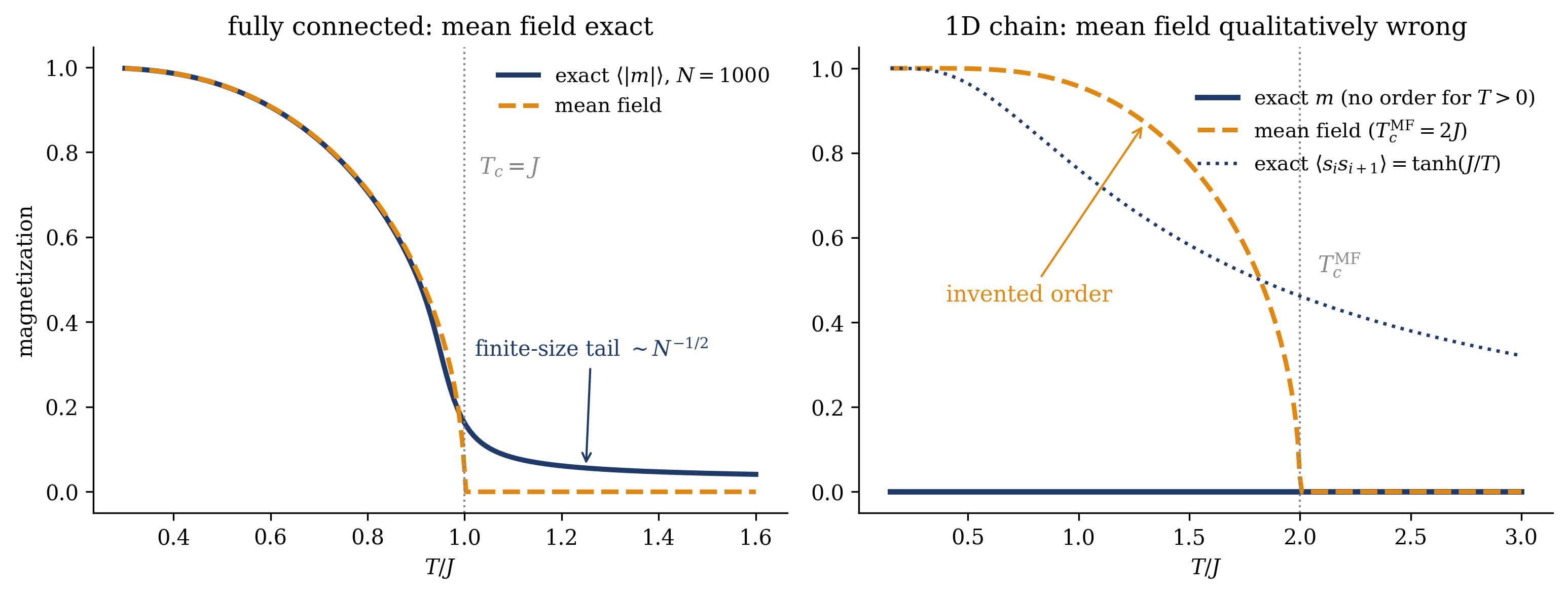
We run the audit rather than assert it — one reassuring case and one damning one, side by side in Figure 10.3.

The reassuring case: the fully-connected model, where the exact answer is computable at real size. The trick is that the energy depends on the configuration only through the total magnetization \(M = \sum_i s_i\), so the \(2^N\)-term partition function collapses onto \(N + 1\) magnetization sectors weighted by binomial degeneracies — Week 1’s “sum over states becomes a sum over macrostates” move, executed exactly. At \(N = 1000\) (\(2^{1000}\) configurations, \(1001\) sectors) the exact \(\langle |m| \rangle\) and the mean-field prediction lie on top of each other through the entire ordered phase — at \(T = 0.5\,J\) they agree to three decimal places (\(0.957\)) — with the only discrepancy a finite-size rounding of width \(\mathcal{O}(N^{-1/2})\) near and above \(T_c\), where the exact finite system’s \(\langle |m| \rangle\) cannot quite vanish. This is mean field’s home turf, verified.

The damning case: the 1D chain, \(z = 2\). Mean field confidently magnetizes at \(T_c^\text{MF} = 2J\). The exact chain (transfer matrix, or Week 1’s two-state machinery applied bond by bond) has \(m = 0\) at every positive temperature — and, drawn alongside, the quantity mean field is constitutionally blind to: the exact nearest-neighbor correlation \(\langle s_i s_{i+1} \rangle = \tanh(\beta J)\), growing smoothly toward \(1\) as the chain cools. Local order builds continuously; long-range order never arrives; and mean field — which cannot tell the two apart, having set all correlations to zero — mistakes the first for the second. The discarded quantity is not a refinement; in one dimension it is the whole story.

model	\(T_c^\text{MF}\)	\(T_c^\text{exact}\)	verdict
1D chain (\(z = 2\))	\(2J\)	\(0\) — no transition	invented order
2D square lattice (\(z = 4\))	\(4J\)	\(2.27\,J\) (Onsager 1944); \(\beta_\text{exp} = \tfrac18\), not \(\tfrac12\)	wrong place, wrong exponent
fully connected (\(J_{ij} = J/N\))	\(J\)	\(J\)	exact (as \(N \to \infty\))

Show code

from scipy.special import gammaln

def exact_fc(T, N=1000, J=1.0):
    k = np.arange(N + 1)
    M = 2 * k - N
    E = -(J / (2 * N)) * (M**2 - N)
    logw = gammaln(N + 1) - gammaln(k + 1) - gammaln(N - k + 1) - E / T
    logw -= logw.max()
    w = np.exp(logw); w /= w.sum()
    return (w * np.abs(M / N)).sum()

def mf_m(T, J0):
    m = 0.999
    for _ in range(5000):
        m = np.tanh(J0 * m / T)
    return m

Ts = np.linspace(0.3, 1.6, 160)
fig, (a1, a2) = plt.subplots(1, 2, figsize=(10.4, 4.0))
a1.plot(Ts, [exact_fc(T) for T in Ts], color=NAVY, lw=2.4,
        label=r"exact $\langle|m|\rangle$, $N=1000$")
a1.plot(Ts, [mf_m(T, 1.0) for T in Ts], color=ORANGE, lw=2.2, ls="--",
        label="mean field")
a1.axvline(1.0, color=GRAY, ls=":", lw=1)
a1.text(1.03, 0.75, r"$T_c = J$", color=GRAY, fontsize=10.5)
a1.annotate(r"finite-size tail $\sim N^{-1/2}$", xy=(1.25, exact_fc(1.25)),
            xytext=(1.02, 0.32), color=NAVY, fontsize=10,
            arrowprops=dict(arrowstyle="->", color=NAVY, lw=1))
a1.set_title("fully connected: mean field exact", fontsize=12)
a1.set_xlabel(r"$T/J$"); a1.set_ylabel("magnetization")
a1.legend(frameon=False, fontsize=9.5)

Ts2 = np.linspace(0.15, 3.0, 300)
a2.plot(Ts2, np.zeros_like(Ts2), color=NAVY, lw=2.6, label=r"exact $m$ (no order for $T>0$)")
a2.plot(Ts2, [mf_m(T, 2.0) for T in Ts2], color=ORANGE, lw=2.2, ls="--",
        label=r"mean field ($T_c^{\rm MF} = 2J$)")
a2.plot(Ts2, np.tanh(1 / Ts2), color=NAVY, lw=1.6, ls=":",
        label=r"exact $\langle s_i s_{i+1}\rangle = \tanh(J/T)$")
a2.axvline(2.0, color=GRAY, ls=":", lw=1)
a2.text(2.08, 0.52, r"$T_c^{\rm MF}$", color=GRAY, fontsize=10.5)
a2.annotate("invented order", xy=(1.3, mf_m(1.3, 2.0)), xytext=(0.4, 0.45),
            color=ORANGE, fontsize=10.5,
            arrowprops=dict(arrowstyle="->", color=ORANGE, lw=1))
a2.set_title("1D chain: mean field qualitatively wrong", fontsize=12)
a2.set_xlabel(r"$T/J$")
a2.set_ylim(-0.05, 1.05)
a2.legend(frameon=False, fontsize=9.5, loc="upper right", bbox_to_anchor=(1.0, 0.95))
fig.tight_layout(); plt.show()

Figure 10.3: The audit, run. Left: the fully-connected model at \(N = 1000\) — the exact \(\langle|m|\rangle\), computed from the \(1001\) magnetization sectors that the \(2^{1000}\)-state sum collapses onto (navy), against the mean-field prediction (orange). The curves coincide through the ordered phase (both \(0.957\) at \(T = 0.5\)); the small exact tail above \(T_c\) is finite-size rounding of order \(N^{-1/2}\), vanishing as \(N \to \infty\). Mean field is exact here. Right: the 1D chain — mean field magnetizes at \(T_c^{\mathrm{MF}} = 2J\) (orange); the exact chain never does (\(m = 0\) for all \(T > 0\), navy). The dashed curve is what mean field cannot see: the exact nearest-neighbor correlation \(\langle s_i s_{i+1}\rangle = \tanh(J/T)\), building smoothly while long-range order never arrives. Mistaking local correlation for global order is precisely the error of setting correlations to zero.

Mean field predicts order from an approximation — and misplaces it; the discrepancy identifies where next week’s corrections are needed.

The tutorial (16–18, Ph12 106) is computation-led: three treatments of one small Ising lattice, side by side: exact enumeration (the truth, affordable only because the lattice is small — Week 3’s ledger set the ceiling), mean field (cheap, deterministic, correlations identically zero), and Monte Carlo sampling (the other road out of an intractable \(Z\), introduced here two weeks before Module 3 makes it a subject). Today’s lecture provides the complete theory of where the three agree and where the mean-field gap opens. The comparison is run in the room by the groups, on their own machines, once each group has written down where it expects the gap to appear.

Take-home 3

Run, the audit confirms the theory: on the fully-connected model mean field coincides with the exact sector-sum answer through the ordered phase; on the 1D chain it magnetizes at \(2J\) while the truth stays disordered forever, mistaking smoothly growing local correlation (\(\tanh \beta J\) — the quantity it set to zero) for long-range order. The gap is the discarded correlations, largest where fluctuations dominate — and where mean field fails is where variational inference will need corrections.

10.6 Outlook: corrections, and the other road

Module 2’s first method now stands complete. A variational approximation, minimizing a bound, predicted collective order, located it at \(T_c = J_0\), gave the transition a universal shape, and founded the language — order parameter, symmetry breaking, Landau landscape — in which this course discusses every collective phenomenon it meets, from Week 2’s memory collapse (a first-order cousin: the order parameter jumped, where today’s grew continuously) to the transitions that lie ahead in sampling dynamics and training. But the method’s one structural act — setting correlations to zero — over-predicts order everywhere, catastrophically so in low dimension, and no optimization within the factorized family can repair it.

Week 6 addresses this directly. If the disease is discarded correlations, the cure is to put them back, systematically. Two restorations, named now and derived next week. The TAP equations — Thouless, Anderson, and Palmer (1977), the same lineage as Week 2’s spin-glass machinery — add to the mean-field equation the leading fluctuation correction, the Onsager reaction term: the part of a spin’s local field that is merely its own influence reflected back by its neighbors, which honest bookkeeping must subtract. And belief propagation — message passing on the interaction graph — generalizes the variational family from independent sites to consistent pairs, is exact on trees, and comes with its own free energy (Bethe’s) standing where Gibbs–Bogoliubov stood today. Both are still road one: approximate the distribution, bound or estimate the free energy, restore correlations order by order.

The tutorial’s third method — Monte Carlo — does not approximate \(p\) at all; it samples it, trading determinism and speed for asymptotic exactness and avoiding \(Z\) entirely. That road is Module 3’s subject, three weeks from now; today’s comparison is an introduction. The course’s three strategies for the partition function remain: bound the free energy (Module 2), sample the distribution (Module 3), and eliminate the normalizer from the gradient (Week 10).