15 Markov chain Monte Carlo: sampling what you cannot normalize

15.1 The other road

Module 2 faced the intractable partition function and approximated the distribution: bounded it with a factorized family (Week 5), corrected the bound (Chapter 11), passed messages on the graph (Chapter 12), and finally decoupled it into a trainable latent-variable model (Chapter 14). Every one of those methods lives with \(Z\) and manages it — deterministically, with a bias fixed by the chosen family. Module 3 opens the road Week 5’s dichotomy left deliberately untaken: do not approximate \(p\) at all — sample it.

The fact that makes this possible is the simplest of the course’s escapes from \(Z\), and we state it carefully. To evaluate \(p(x) = e^{-\beta E(x)}/Z\) you need \(Z\), and that is hopeless. But to sample, you never need the probability of any single state; you only ever need to compare two, and in the ratio

\[ \frac{p(x')}{p(x)} \;=\; \frac{e^{-\beta E(x')}/Z}{e^{-\beta E(x)}/Z} \;=\; e^{-\beta\,\Delta E}, \qquad \Delta E = E(x') - E(x), \]

the partition function cancels. Everything that follows today is the systematic exploitation of that cancellation: you can draw samples from a distribution you cannot normalize. The course has now met three distinct ways of defusing \(Z\) — Module 1 dodged its parameter-gradient (contrastive divergence), Module 2 bounded its logarithm (the variational free energy), and Module 3 makes it cancel — with the fourth and final way, removal (\(\nabla_x \log Z = 0\)), still two weeks out.

The history closes a loop the course opened on day one. In 1953, at Los Alamos, Nicholas Metropolis, Arianna and Marshall Rosenbluth, and Augusta and Edward Teller published Equation of State Calculations by Fast Computing Machines (Metropolis et al. 1953) — the “fast computing machine” being the MANIAC, one of the first electronic computers, and the calculation being the equilibrium properties of a fluid of hard disks that no closed form could touch. Their idea — walk through configuration space, accepting each proposed move with a probability built from the Boltzmann ratio — is Markov chain Monte Carlo, and it now runs everywhere from lattice QCD to Bayesian statistics to the negative phase of Week 3’s Boltzmann machines. Hastings (1970) generalized it; the modern world computes with it.

Module 3 is defined as much by its cost as by its trick. Sampling is asymptotically exact — run the chain forever and the answers converge to the truth, no family bias, no bound looseness. What it pays instead is time: the chain must mix — forget its initialization and visit configuration space with the right frequencies — and mixing is slow precisely where this course’s landscapes are interesting: near phase transitions, and in the rugged terrain of Weeks 2 and 6. Module 3 swaps the normalization obstruction for the sampling one; today makes both the trick and the price precise.

Take-home 1

To sample \(p \propto e^{-\beta E}\) you never need \(Z\) — only energy differences, because \(Z\) cancels in every ratio \(p(x')/p(x) = e^{-\beta \Delta E}\). Sampling is Module 3’s road out of the normalization obstruction Module 2 bounded; its price is mixing.

15.2 Approximate versus sample

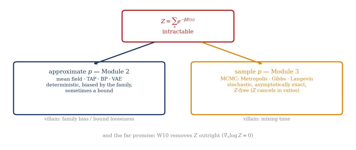
The module map frames the fork (Figure 15.1). Road one — Module 2 — replaces \(p\) by the best member of a tractable family: deterministic, fast, sometimes armed with a bound, and biased forever by whatever the family cannot express (the factorized ansatz never contained a correlation, no matter how long you optimized). Road two — this module — builds a stochastic process whose visits are draws from \(p\): no family, no bias in the limit, and instead a stochastic error that shrinks with simulation time — if the process equilibrates. The choice is deterministic-and-biased against stochastic-and-exact-eventually; the course will need both, and Module 4 will need them married.

Figure 15.1: The two roads out of an intractable \(Z\). Module 2 approximated the distribution — mean field, TAP, message passing, the VAE — deterministic and biased by the chosen family, sometimes with a bound. Module 3 samples it: Markov chain Monte Carlo is stochastic, asymptotically exact, and \(Z\)-free, because the normalizer cancels in every ratio the algorithm ever uses. Each road has its own obstruction: family bias on one, mixing time on the other — and Week 10’s score matching still waits at the bottom, where \(Z\) is neither bounded nor canceled but removed.

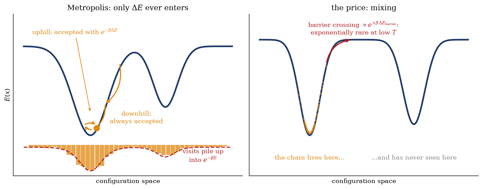
Figure 15.2 draws the method before the mathematics. Left: a walker on an energy landscape takes proposed steps — downhill steps always accepted, uphill steps accepted with probability \(e^{-\beta \Delta E}\) — and the histogram of its visits piles up, over time, into exactly \(e^{-\beta E}\): the Boltzmann distribution, assembled from nothing but local energy differences. Right: the same walker at low temperature, trapped in one basin behind a barrier it crosses only with exponentially small probability — sampling that basin faithfully, having never seen the rest of configuration space. The left panel is the theorem we now prove; the right is the price we then pay.

Figure 15.2: The central picture of Module 3’s opening. Left: the Metropolis walker — downhill proposals always accepted, uphill ones accepted with probability \(e^{-\beta\Delta E}\) — and the histogram of its visits (orange) converging onto \(e^{-\beta E}\) (red dashed): the Boltzmann distribution sampled without \(Z\) ever being computed. Right: the price. At low temperature a barrier is crossed only with probability \(\sim e^{-\beta\,\Delta E_{\text{barrier}}}\) per attempt; the chain samples its home basin perfectly and has never seen the other one. Equilibration within a basin is not equilibration.

15.3 The engine: detailed balance and the Metropolis rule

Setup. We want a stochastic process on configuration space — a Markov chain, specified by transition probabilities \(W(x \to x')\) — whose long-run visit frequencies are \(p(x) \propto e^{-\beta E(x)}\), built using only the ratio \(e^{-\beta \Delta E}\). The design condition is stationarity: if the chain’s states are distributed as \(p\) at one step, they must remain so at the next,

\[ \sum_x p(x)\, W(x \to x') \;=\; p(x') \quad \text{for all } x'. \]

(That a well-behaved chain then converges to this \(p\) from any start — uniqueness of the stationary distribution under irreducibility and aperiodicity, Perron–Frobenius — is the same bookkeeping we took as read for Glauber in Section 5.3, and the script keeps it in the margin. Design is today’s business; convergence rate is the second half of the lecture.)

Detailed balance. Stationarity is a global condition — a sum over all states, awkward to engineer directly. The workhorse is a local, pairwise condition that implies it:

\[ \boxed{\; p(x)\, W(x \to x') \;=\; p(x')\, W(x' \to x) \quad \text{for all pairs } x, x' \;} \tag{15.1}\]

detailed balance \(\Rightarrow\) \(p\) stationary

— detailed balance: at equilibrium, probability flows equally in both directions across every pair of states, not just in aggregate. The implication is one line — sum both sides over \(x\), and \(\sum_x W(x' \to x) = 1\) collapses the right side:

\[ \sum_x p(x)\, W(x \to x') \;=\; p(x') \sum_x W(x' \to x) \;=\; p(x'). \]

You have seen this condition before, doing exactly this job: it is what gave Glauber dynamics its Boltzmann stationary law in Section 5.3, there checked for one specific flip rule. Today it is promoted from a property we verified to a design principle we build from. (One margin note, made precise at the end of this section: detailed balance is sufficient, not necessary — valid and sometimes faster chains exist that break it. It is the standard tool because it is the checkable one.)

The Metropolis rule. Split each transition into a proposal and an acceptance: \(W(x \to x') = g(x \to x')\, A(x \to x')\), with \(g\) symmetric (\(g(x \to x') = g(x' \to x)\) — flip a random spin, jiggle a coordinate) and the acceptance chosen as

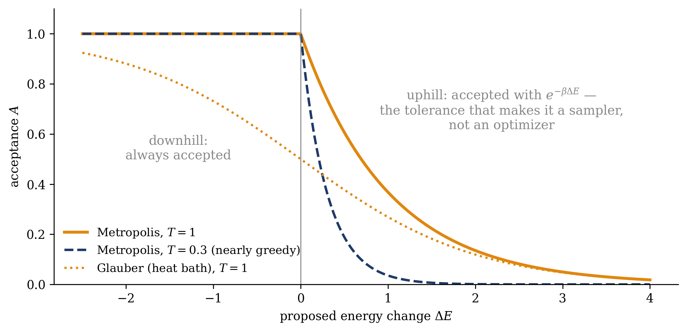
\[ \boxed{\; A(x \to x') \;=\; \min\!\big( 1,\; e^{-\beta\, \Delta E} \big) \;} \tag{15.2}\]

Metropolis acceptance

— accept every downhill move; accept an uphill move with probability \(e^{-\beta \Delta E}\) (Figure 15.3). The detailed-balance check, which completes the derivation, takes two lines. With symmetric \(g\),

\[ p(x)\, g\, A(x \to x') \;=\; g\, \min\!\big( p(x),\, p(x') \big) \;=\; p(x')\, g\, A(x' \to x), \]

because \(p \min(1, p'/p) = \min(p, p')\) — an expression manifestly symmetric under \(x \leftrightarrow x'\), so Equation 15.1 holds by inspection. And the algorithm consumed only one thing: \(p\) entered only through the ratio \(p(x')/p(x) = e^{-\beta\Delta E}\). \(Z\) never appears. The chain’s visit frequencies converge to the full, correctly normalized Boltzmann distribution — normalizer included — and the normalizer was never computed, only canceled. One local rule, using one energy difference per step, samples a globally intractable distribution exactly.

Two standard extensions complete the design. For asymmetric proposals, Hastings (1970) rebalances the acceptance, \(A = \min\big(1, \frac{p(x')\,g(x' \to x)}{p(x)\,g(x \to x')}\big)\) — still a ratio, \(Z\) still gone. And proposing from an exact conditional distribution (resample one variable given all others) makes the Hastings ratio identically one — accept always: the Gibbs sampler (Geman and Geman 1984), which you have been running since Week 3, because the RBM’s block Gibbs (Section 6.3) is precisely this with whole layers as the resampled blocks. Glauber’s flip rule, likewise, is just a different valid acceptance function (\(1/(1 + e^{\beta\Delta E})\) — the “heat bath” choice, gentler than Metropolis’s \(\min\), satisfying the same detailed balance). One principle generates a family of algorithms.

Sufficient, not necessary: the adjoint kernel. The precise statement identifies what stationarity actually requires — and introduces one of the module’s central objects (Welling, Lu, and Holdijk 2026, ch. 11 on Markov chain Monte Carlo). We claim that \(p\) is stationary under \(W\) if and only if there exists a second transition probability \(W^\dagger\) — the adjoint kernel, nonnegative and normalized — satisfying the generalized balance relation

\[ p(x)\, W(x \to x') \;=\; p(x')\, W^\dagger(x' \to x) \quad \text{for all pairs } x, x'. \tag{15.3}\]

generalized balance: stationarity’s exact requirement

One direction is the same one-line sum as before: if such a \(W^\dagger\) exists, summing Equation 15.3 over \(x\) gives \(\sum_x p(x)\, W(x \to x') = p(x') \sum_x W^\dagger(x' \to x) = p(x')\), which is stationarity. For the converse there is only one candidate — solve Equation 15.3 for

\[ W^\dagger(x' \to x) \;=\; \frac{p(x)\, W(x \to x')}{p(x')}, \]

manifestly nonnegative, and check that it is normalized:

\[ \sum_x W^\dagger(x' \to x) \;=\; \frac{1}{p(x')} \sum_x p(x)\, W(x \to x'), \]

which equals one for every \(x'\) exactly when \(p\) is stationary. The constructed \(W^\dagger\) is a genuine transition kernel precisely when the chain has \(p\) as its stationary law, and the equivalence is proved. Detailed balance is the special case \(W^\dagger = W\): the chain is its own adjoint.

The adjoint has a physical reading that the course will lean on. By construction, \(W^\dagger(x' \to x)\) is the probability that a stationary chain sitting at \(x'\) arrived from \(x\) — Bayes’ rule applied to one step — so \(W^\dagger\) is the chain watched in reverse. Detailed balance then says the film run backwards is statistically indistinguishable from the film run forwards: no pair of states carries a net probability current, which is the defining property of equilibrium. Generalized balance permits more: \(W^\dagger \neq W\), probability circulating around closed loops, every state’s total inflow and outflow balancing while individual pairs carry steady current. Such a chain is stationary but irreversible — a nonequilibrium steady state, the same object whose circulating currents reappear in Week 9’s anisotropic SGD — and irreversibility is not a defect: the persistent current stirs the state space rather than diffusing through it, which is why deliberately non-reversible chains can mix faster than any detailed-balance competitor built from the same moves. You have, in fact, been running one since Week 3: fixed-scan Gibbs — the RBM’s \(v \to h \to v\) ladder — satisfies detailed balance in each half-step but not in their composition (its adjoint is the scan run in the opposite order), and it leaves \(p\) invariant all the same. Why, then, does detailed balance remain the standard tool? Because normalizing \(W^\dagger\) is exactly as global a check as stationarity itself — a sum over all states — while detailed balance is verified pair by pair, from energy differences alone. Design locally with Equation 15.1, knowing the license Equation 15.3 grants is wider; Week 10 will use that license out of equilibrium, where the marginals themselves change in time and the reversed kernel becomes the generative object.

Show code

dE = np.linspace(-2.5, 4, 500)
fig, ax = plt.subplots(figsize=(8.0, 3.9))
ax.plot(dE, np.minimum(1, np.exp(-dE / 1.0)), color=ORANGE, lw=2.4,
        label=r"Metropolis, $T = 1$")
ax.plot(dE, np.minimum(1, np.exp(-dE / 0.3)), color=NAVY, ls="--", lw=2.0,
        label=r"Metropolis, $T = 0.3$ (nearly greedy)")
ax.plot(dE, 1 / (1 + np.exp(dE / 1.0)), color=ORANGE, ls=":", lw=1.8,
        label=r"Glauber (heat bath), $T = 1$")
ax.axvline(0, color=GRAY, lw=0.8)
ax.text(-1.4, 0.5, "downhill:\nalways accepted", color=GRAY, fontsize=10.5, ha="center")
ax.text(2.3, 0.62, "uphill: accepted with $e^{-\\beta\\Delta E}$ —\n"
        "the tolerance that makes it a sampler,\nnot an optimizer", color=GRAY,
        fontsize=10.5, ha="center")
ax.set_xlabel(r"proposed energy change $\Delta E$")
ax.set_ylabel(r"acceptance $A$")
ax.set_ylim(0, 1.1)
ax.legend(frameon=False, fontsize=9.5, loc="lower left")
fig.tight_layout(); plt.show()

Figure 15.3: The Metropolis acceptance Equation 15.2 against the proposed energy change, at two temperatures, with Glauber’s heat-bath rule (Section 5.3) alongside for the warm case. Downhill moves (\(\Delta E < 0\)) are always accepted; uphill moves survive with probability \(e^{-\beta\Delta E}\) — the uphill tolerance that distinguishes a *sampler* from Week 2’s greedy descent, and the only place temperature enters the algorithm. Cool the chain and the tolerance narrows toward pure descent (navy dashed); both acceptance functions satisfy detailed balance with respect to the same Boltzmann distribution, Metropolis simply accepting more.

15.4 We have been sampling since Week 3 — and the price is mixing

The unification, first. The method is not new to this course, but it now gets its name. Glauber dynamics — Week 3’s stochastic flip rule, from which the Boltzmann machine was built — is single-spin MCMC with the heat-bath acceptance. The RBM’s block Gibbs ladder is the Gibbs sampler, layer by layer. And now the result Week 3 could only promise: contrastive divergence is a truncated Markov chain — a sampler deliberately run \(k\) steps from the data instead of to equilibrium — and that is the entire content of its bias. In Section 6.4 we quantified the CD-\(k\) gap and watched it decay with \(k\); today’s language names the mechanism: an unequilibrated chain samples the wrong distribution, so the negative phase it estimates is systematically off, by exactly the amount the chain has failed to mix — a corollary of today’s framework.

The price: mixing. Everything above says the chain converges; none of it says when. Three costs follow, in ascending order of severity. First, MCMC samples are correlated: consecutive states differ by one accepted move, so a run of \(N\) steps carries not \(N\) independent draws but roughly \(N/(2\tau)\), where \(\tau\) is the autocorrelation time — the number of steps the chain needs to forget itself. Second, the chain needs burn-in: samples taken before stationarity is reached are draws from the wrong distribution and must be discarded (CD’s bias again, this time as a lab habit). Third — the main obstruction — \(\tau\) itself can blow up. It does so in exactly the two regimes this course keeps meeting. Near a critical point, fluctuations become system-spanning while the dynamics stays local, and \(\tau\) grows as a power of the correlation length (critical slowing down — the worked example below measures it); physics has cures here (cluster algorithms that flip correlated islands wholesale — named for the script, not developed). In rugged, glassy landscapes — Week 2’s overloaded memory, Week 6’s spin glass — barriers are extensive, crossing times are exponential, and below the glass transition ergodicity breaks: the chain is confined to one valley of many, and no polynomial patience rescues it. For the models this course cares about, Figure 15.2’s right panel is the typical terrain rather than a pathology.

A question from Week 3 is now settled: normalization and sampling are two distinct obstructions. Module 2 fought the first — \(Z\), the normalizer — by bounding and approximating. Module 3 makes the first cancel outright, and inherits the second: mixing. Neither implies the other (a perfectly known \(Z\) would not flatten a single barrier), and the map of the field keeps them separate. MCMC yields samples and ratios, never \(Z\) itself — if you genuinely need the normalizer (to compare models, to report a likelihood), sampling alone is not enough, and the machinery that extracts free energies from chains (thermodynamic integration, annealed importance sampling) is Week 11’s, where it arrives in the language of nonequilibrium thermodynamics.

Trap

A chain that has not mixed samples the wrong distribution — and it will not warn you. MCMC’s samples are correlated (effective sample size \(N/(2\tau)\), not \(N\)), require burn-in, and are only asymptotically exact given equilibration. An unmixed chain produces smooth, convergent-looking, reproducibly wrong averages — it is why contrastive divergence is biased (Section 6.4), and why every MCMC result owes its reader an autocorrelation time. And do not over-credit the trick: \(Z\) cancels in ratios, but MCMC never gives you \(Z\) — samples are not normalizers (that debt is settled in Week 11).

Take-home 2

Glauber dynamics, block Gibbs, and contrastive divergence are all MCMC — and CD is biased precisely because its chain is deliberately not equilibrated. The price of \(Z\)-free sampling is mixing: correlated samples (\(N_\text{eff} \approx N/(2\tau)\)), mandatory burn-in, autocorrelation times that diverge at critical points and grow exponentially in glassy landscapes. Normalization and mixing are distinct obstructions; Module 3’s subject is the second.

15.5 Example: Metropolis on the two-dimensional Ising model

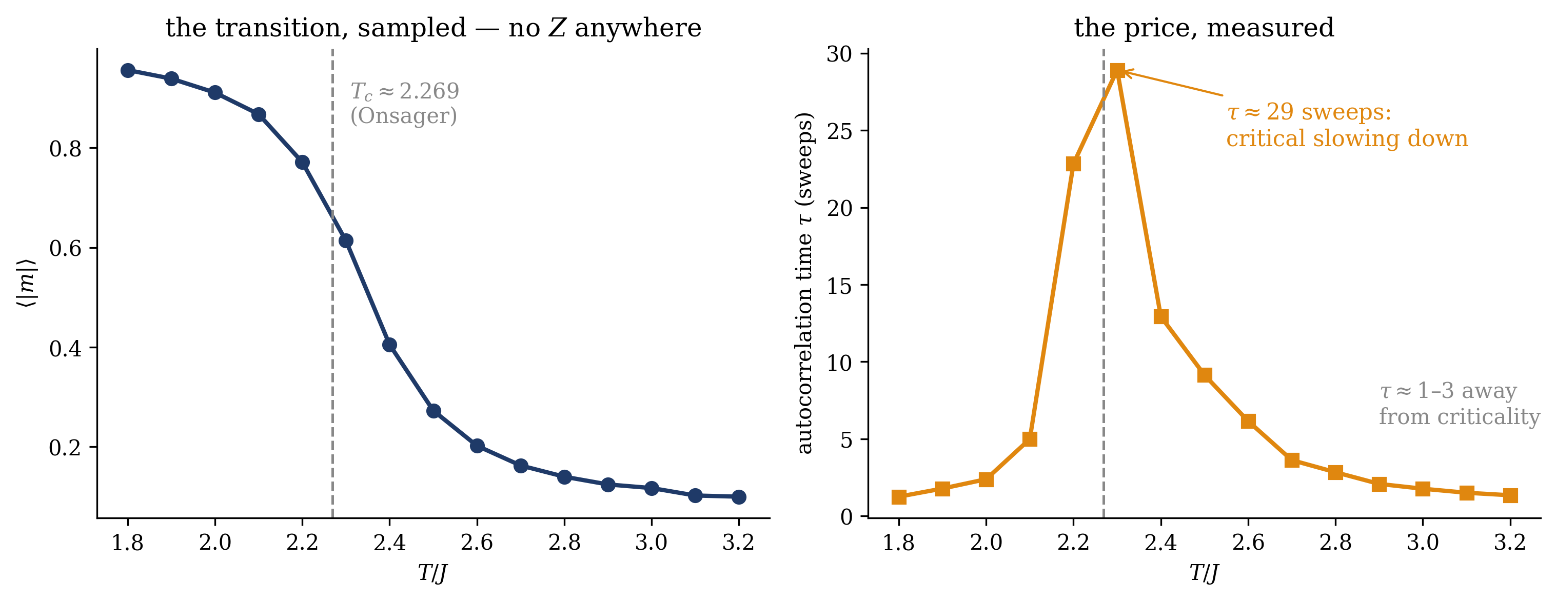
One chain makes both faces of the lecture visible — the method’s power and its cost. Run checkerboard Metropolis on a \(24 \times 24\) Ising lattice (the two sublattices updated in alternating half-sweeps, a vectorized equivalent of single-site updates) across the temperature range straddling Onsager’s exact critical point \(T_c = 2/\log(1 + \sqrt{2}) \approx 2.269\) (Onsager 1944), and measure two things: the magnetization, and the autocorrelation time of its time series (Figure 15.4).

The magnetization curve shows what sampling achieves. The full phase transition — the ordered branch, the collapse at \(T_c\), the disordered tail — emerges from a walker that only ever computed local energy differences: no \(Z\), no free energy, no \(2^{576}\)-term sum, just \(\min(1, e^{-\beta\Delta E})\) applied a few million times. Where Week 5 obtained this curve from a variational bound (with a manufactured transition in the wrong place) and the exact treatments of Weeks 1–2 needed enumerability, the sampler simply visits the truth. And it is genuinely the truth: on a \(4\times 4\) lattice, where all \(65{,}536\) states can be enumerated, the same chain reproduces the exact \(\langle |m| \rangle\) to a few parts in a thousand:

\(T\)	exact \(\langle\|m\|\rangle\) (\(4\times4\), enumerated)	MCMC estimate
\(2.0\)	\(0.9189\)	\(0.9193\)
\(2.5\)	\(0.7647\)	\(0.7606\)
\(3.0\)	\(0.6013\)	\(0.5977\)

The autocorrelation panel shows the cost. Away from the transition, \(\tau \approx 1\)–\(3\) sweeps — consecutive configurations decorrelate almost immediately, and every sweep is nearly a fresh sample. Approaching \(T_c\), the time series becomes sticky — long correlated excursions as system-spanning fluctuation patterns rearrange through single spin flips — and \(\tau\) spikes to \(\approx 29\) sweeps, a twenty-fold collapse in effective sample size, at fixed computational cost. Critical slowing down is visible directly, and it scales: on larger lattices the peak grows as a power of the system size, and in the glassy landscapes of Weeks 2 and 6 the analogous times are exponential. The sampler is exact when it mixes; the plot shows where mixing fails — where the physics is most interesting.

Show code

def metropolis_ising(L, T, sweeps, burn, rng):
    s = rng.choice([-1, 1], size=(L, L))
    mask = (np.indices((L, L)).sum(axis=0) % 2).astype(bool)
    ms = np.empty(sweeps)
    for t in range(burn + sweeps):
        for sub in (mask, ~mask):                      # checkerboard half-sweeps
            nb = (np.roll(s, 1, 0) + np.roll(s, -1, 0) +
                  np.roll(s, 1, 1) + np.roll(s, -1, 1))
            dE = 2 * s * nb                            # flip cost, all sites at once
            acc = (rng.random((L, L)) < np.exp(-dE / T)) & sub
            s = np.where(acc, -s, s)                   # Metropolis: min(1, e^{-dE/T})
        if t >= burn:
            ms[t - burn] = abs(s.mean())
    return ms

def tau_int(x, c=5):
    """integrated autocorrelation time, automatic windowing."""
    x = x - x.mean()
    n = len(x)
    f = np.fft.rfft(x, 2 * n)
    acf = np.fft.irfft(f * np.conj(f))[:n].real
    acf /= acf[0]
    tau = 0.5
    for M in range(1, n // 2):
        tau += acf[M]
        if M >= c * tau:
            return max(tau, 0.5)
    return tau

rng = np.random.default_rng(1)
L = 24
Ts = np.linspace(1.8, 3.2, 15)
mm, tt = [], []
for T in Ts:
    series = metropolis_ising(L, T, sweeps=10000, burn=1500, rng=rng)
    mm.append(series.mean())
    tt.append(tau_int(series))

Tc = 2 / np.log(1 + np.sqrt(2))
fig, (a1, a2) = plt.subplots(1, 2, figsize=(10.4, 4.0))
a1.plot(Ts, mm, "o-", color=NAVY, lw=2)
a1.axvline(Tc, color=GRAY, ls="--", lw=1.2)
a1.text(Tc + 0.04, 0.85, r"$T_c \approx 2.269$" "\n(Onsager)", color=GRAY, fontsize=10)
a1.set_xlabel(r"$T/J$"); a1.set_ylabel(r"$\langle |m| \rangle$")
a1.set_title("the transition, sampled — no $Z$ anywhere", fontsize=12)
a2.plot(Ts, tt, "s-", color=ORANGE, lw=2)
a2.axvline(Tc, color=GRAY, ls="--", lw=1.2)
a2.annotate(rf"$\tau \approx {max(tt):.0f}$ sweeps:" "\ncritical slowing down",
            xy=(Ts[int(np.argmax(tt))], max(tt)), xytext=(2.55, 24),
            color=ORANGE, fontsize=10.5,
            arrowprops=dict(arrowstyle="->", color=ORANGE, lw=1))
a2.text(2.9, 6, r"$\tau \approx 1$–$3$ away" "\nfrom criticality", color=GRAY, fontsize=10)
a2.set_xlabel(r"$T/J$"); a2.set_ylabel(r"autocorrelation time $\tau$ (sweeps)")
a2.set_title("the price, measured", fontsize=12)
fig.tight_layout(); plt.show()

Figure 15.4: The power and its price, on one chain: checkerboard Metropolis on a \(24\times24\) Ising lattice (\(10{,}000\) measurement sweeps per temperature after burn-in). Left: the sampled magnetization \(\langle|m|\rangle(T)\) traces the full phase transition across Onsager’s \(T_c \approx 2.269\) (dashed) — obtained from local energy differences alone, with \(Z\) never computed (and verified against exact enumeration on a \(4\times4\) lattice to a few parts per thousand). Right: the price — the autocorrelation time of the magnetization series spikes from \(\sim 1\) sweep far from criticality to \(\approx 29\) sweeps near \(T_c\): critical slowing down. The effective sample size collapses exactly where the physics is most interesting; in glassy landscapes the same cost becomes exponential.

You can sample a distribution you cannot normalize — \(Z\) cancels in every ratio; what you cannot escape is mixing.

The week continues from here. The warm-up card, due the evening before the next lecture, covers Kirkpatrick, Gelatt, and Vecchi (1983) — ten pages of Science, and a landmark idea-transplant between fields; read it with today’s Metropolis rule in hand, and notice what the authors do to the temperature. In the next lecture we do it deliberately: temperature stops being a fixed parameter and becomes a schedule — run the chain hot to cross barriers, cool it to distill low-energy states — and the derivation-led tutorial takes that machinery to a famously hard optimization problem, then sets it beside a stochastic-gradient sampler of a Bayesian posterior. What those two have to do with each other is for the tutorial to establish. The tutorial requires no devices.

Take-home 3

Metropolis samples the 2-D Ising phase transition without ever computing \(Z\) — and matches exact enumeration where enumeration is possible — but its autocorrelation time spikes twenty-fold at \(T_c\): critical slowing down, the mixing cost made visible. The method is exact when it mixes and silently unreliable when it does not; whether a chain can be trusted is entirely a matter of equilibration.

15.6 Outlook: temperature becomes a tool

Module 3 is open. A fifty-line algorithm samples the distribution whose normalizer was intractable throughout Weeks 3–7, by canceling it in every ratio. The cost is equilibration, purchased in time, at prices that diverge where landscapes become interesting. The next lecture takes the algorithm’s parameter — temperature — and turns it from a parameter into an instrument: at high \(T\) the walker ignores barriers and roams globally; at low \(T\) it commits and refines; and a cooling schedule harvests both, using the Boltzmann distribution’s own concentration onto low-energy states as an optimization principle. That is simulated annealing (Kirkpatrick, Gelatt, and Vecchi 1983) — metallurgy imported into computation — and with it Module 3’s second theme: the dynamics of a sampler as a subject in itself.

Week 9 then delivers the module’s main consequence for machine learning. Stochastic gradient descent — the algorithm training every model in this course’s second half — takes noisy downhill steps on a loss landscape: a proposal (the gradient direction, jittered by the mini-batch) and no explicit acceptance, yet its long-run behavior is that of a Langevin sampler at a temperature set by the learning rate and batch size. Training is sampling; the optimizer is a Metropolis walker with the thermostat hidden in the hyperparameters; and the stationary distribution it samples — which minima it likes, and why flat ones — is a Boltzmann distribution over the loss. The Fokker–Planck machinery for making all of that precise is Week 9’s engine, and it is also — one module later — the mathematical substrate of diffusion models. The spine reads once more, now with three of its four vertebrae in place: Module 1 dodged \(\nabla_\theta \log Z\), Module 2 bounded \(\log Z\), Module 3 makes \(Z\) cancel — and Week 10 removes it.