Core (~1 h).Hopfield (1982) — the founding paper, five pages, and remarkably readable. Read all of it: the content-addressable-memory framing, the storage prescription, the update rule, and even a numerical capacity estimate are already there. This is also the source for this week’s tutorial warm-up, so the hour is spent twice. Alongside it, MacKay (2003), Ch. 42 — the inference-side telling of the same model, associative memory as an error-correcting code, with the convergence argument done cleanly (freely available online).
Optional background.Hertz, Krogh, and Palmer (1991), Ch. 2–3, the textbook treatment of the Hopfield model, whose logic this chapter follows closely; Amit (1989), Ch. 1–2, for the attractor picture developed at length by one of the people who solved the model; Nishimori (2001), Ch. 7, for associative memory in the spin-glass language Module 2 will need; and the energy-based-model sections of Mehta et al. (2019) for the machine-learning vocabulary this module now makes precise.
Prerequisite reminder. The Ising model — Hamiltonian, ferromagnetic ordering, single-spin-flip dynamics — is assumed from master’s statistical mechanics. What is new is not the spin system; it is the inversion of the problem: choosing the couplings so that the minima sit where we want them, and reading relaxation as computation.
3.1 How can a physical system remember?
Start from an everyday observation so familiar it goes unnoticed. You recognize a friend from a quarter of a face in bad light. You complete “to be or not to —” without consulting an index. In both cases a fragment of the content retrieves the whole — no address, no lookup table, no exact match required. Whatever implements this in the brain, it is nothing like the random-access memory in a computer, where the address is the mechanism and a single corrupted address bit fetches garbage. The question this week answers is how a physical system — neurons, spins, anything with an energy — can remember in the first sense. The question carries weight: the 2024 Nobel Prize in Physics went to John Hopfield and Geoffrey Hinton “for foundational discoveries and inventions that enable machine learning with artificial neural networks,” and the two objects the citation points at are precisely the subjects of Weeks 2 and 3, honored as physics. Today we meet the first of them, and we will find that it is an Ising model put to a new purpose.
The idea has a lineage, and we trace it because Hopfield’s contribution was a fusion, not an invention from nothing — three ingredients from three fields that lay separately for decades. McCulloch and Pitts (1943) modeled the neuron as a binary threshold unit and showed that networks of such units can compute logical functions: the unit of neural computation existed by 1943, but the treatment was logical, with nothing collective in it — no robustness, no storage, no dynamics. Hebb (1949) supplied a storage prescription in prose: neurons that fire together strengthen their connection — a learning rule stated decades before it had a mathematical home. Little (1974) made the physics mapping explicit, casting neural firing as an Ising system with synchronous, parallel dynamics. And the missing ingredient arrived from condensed matter, from a direction that had nothing to do with brains: the spin-glass theory of Edwards and Anderson (1975) and Sherrington and Kirkpatrick (1975) made disordered couplings a first-class object of statistical mechanics. Rugged energy landscapes with many metastable minima stopped being a pathology to average away and became a structure to study — and a landscape with many minima is exactly what a memory needs, one minimum per stored item.
Hopfield (1982) fused the three. Take McCulloch–Pitts threshold units; couple them with an Ising energy whose couplings are chosen by Hebb’s rule from the data; update them asynchronously, one at a time, with symmetric couplings — and, as we prove below, the dynamics rolls strictly downhill on an energy landscape whose minima are the stored patterns. Memory becomes an attractor; recall becomes relaxation. Three years later, Amit, Gutfreund, and Sompolinsky (1985) did to this model what physicists do to any model — computed its phase diagram — and found that associative memory survives up to a sharp critical storage load. That calculation is the next lecture; the spin-glass machinery inside it, this course meets through its modern mean-field descendants in Module 2.
A memory is not a stored record but a dynamical attractor — and the same mathematics that makes a ferromagnet remember its magnetization direction can be engineered to remember a photograph.
Through Week 1, the energy \(E(x)\) was given, and everything flowed forward from it: given \(E\), maximum entropy delivered \(p = e^{-\beta E}/Z\) (Section 1.4), and the saddle-point toolkit computed with it (Chapter 2). Today, for the first time, the direction inverts — we choose\(E\) — and one absence is worth noticing: nothing in this lecture mentions \(Z\). The network below runs deterministically, at zero temperature; there are no probabilities to normalize. This is the first of only two stretches in the course — this week and Week 4 — where the partition function plays no role. Week 3 heats this same network back up, and \(Z\) returns as the obstruction that training must confront.
Take-home 1
Associative memory is an energy landscape used as a computer: stored patterns are engineered minima, cues are initial conditions, retrieval is relaxation. The Hopfield network is the Ising model with its couplings chosen by data — the first energy-based model.
3.2 From lookup to attractor
Two dichotomies organize the week.
The first is address versus attractor. A conventional memory implements the map address → contents; it is exact, fast, and brittle — corrupt one address bit and you retrieve an unrelated word. An associative (or content-addressable) memory implements the map partial contents → full contents; the query is a corrupted fragment of the thing itself, and the corruption is not fatal but repaired by the dynamics. There is an engineering reading of this that MacKay develops and we only flag: an associative memory is an error-correcting code, with the basin of attraction playing the role of the code’s correction radius (MacKay 2003).
The second dichotomy is the one that defines Module 1: measured versus designed energy. Physics traditionally receives its Hamiltonian from nature and asks what states it produces. Hopfield inverts the question: given the desired states \(\{\xi^\mu\}\) — the memories — what energy has them as its minima? This inverse problem is precisely what Week 1 promised under the slogan “learning is shaping an energy landscape,” and everything in this module is a progressively better answer to it: Hebb’s one-shot rule today, gradient-trained Boltzmann machines in Week 3, modern Hopfield networks in Week 4.
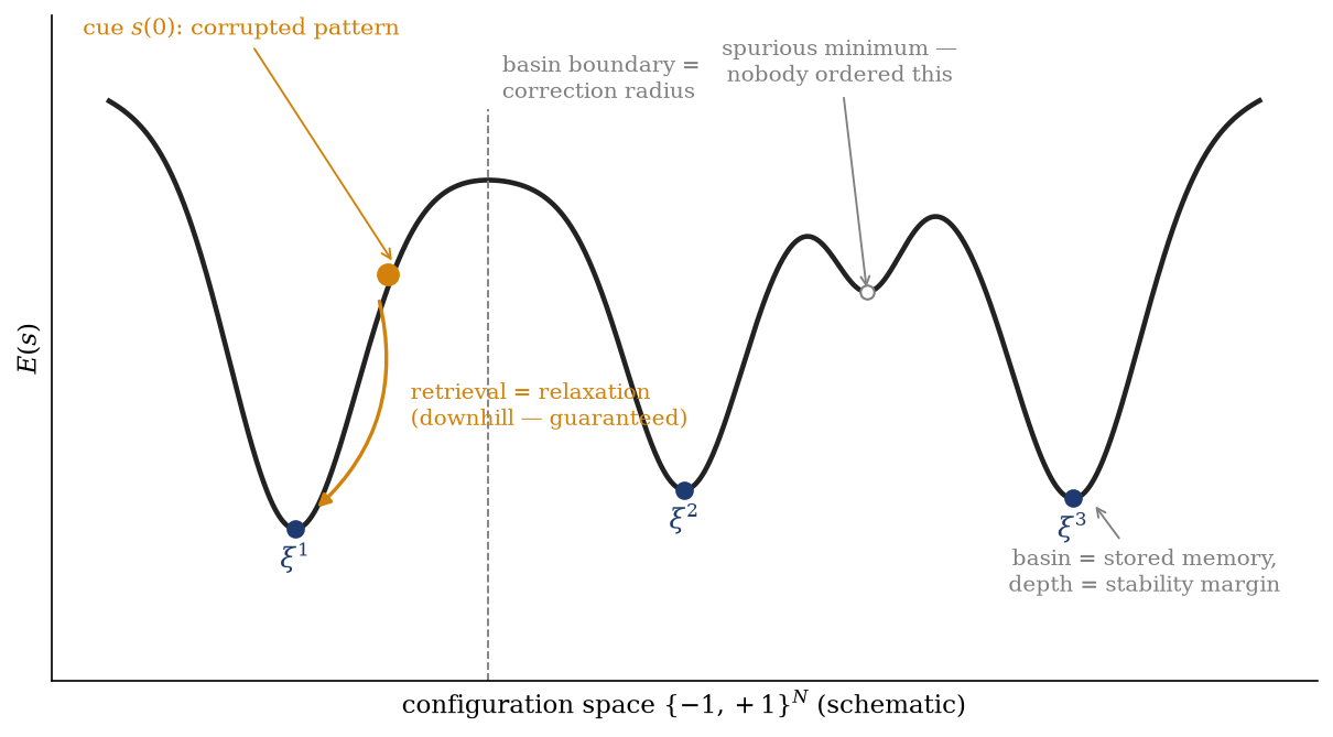
Figure 3.1 draws the central picture, one the course keeps returning to: an energy landscape over configuration space, where each stored pattern sits in an engineered basin, a corrupted cue starts partway up a basin wall, and retrieval is the roll downhill. The picture rests on three concrete requirements: ① a dynamics that “rolls downhill” even though our variables are discrete spins with no gradient; ② a proof that this dynamics reaches a minimum and halts (the derivation of Section 3.4); ③ a recipe for placing the minima at the data — Hebb’s rule. The figure also shows a minimum nobody ordered, reflecting a general property of designed landscapes rather than a drawing error.
Figure 3.1: The central picture of Module 1: memory as an energy landscape. Stored patterns \(\xi^1, \xi^2, \xi^3\) are engineered minima; a corrupted cue \(s(0)\) is an initial condition partway up a basin wall; retrieval is relaxation to the basin’s bottom, and the basin boundary sets how much corruption is correctable. The dynamics is guaranteed to run downhill (the Lyapunov theorem of Section 3.4) — but the landscape also contains spurious minima that nobody ordered, a point we return to at the end of the chapter.
3.3 The model: neurons as spins
Each object below carries two names — one from physics, one from machine learning — since the course works at their interface.
Take \(N\) binary neurons\(s_i = \pm 1\), firing or quiet — which we read, with no modification whatsoever, as \(N\) Ising spins, up or down. The network state \(s = (s_1, \dots, s_N)\) is a corner of the hypercube \(\{-1, +1\}^N\): a configuration in exactly the sense of Week 1’s symbol table, \(x \leftrightarrow s\), and we will use \(s\) whenever the configuration is a neural state. Each neuron feels a local field — in machine-learning language, a pre-activation —
\[
h_i = \sum_{j} J_{ij}\, s_j,
\]
where the couplings \(J_{ij}\) are, in the other dialect, the weights of the network (\(w_{ij}\) in most of the ML literature; we keep \(J\) and the physics conventions). The dynamics is the simplest thing the local field permits: pick a neuron — asynchronously, one at a time, in random order — and align it with its field,
Thresholds are set to zero throughout — for the symmetric \(\pm 1\) patterns we store, they buy nothing — which also spares us a notation clash, since the course reserves \(\theta\) for model parameters.
Two structural assumptions complete the model, and we state them as deliberate choices rather than habits, because the next section shows exactly what each one buys: the couplings are symmetric, \(J_{ij} = J_{ji}\), and carry no self-coupling, \(J_{ii} = 0\). Under these assumptions we associate to the network the energy
— an infinite-range Ising Hamiltonian with heterogeneous couplings. As an object, nothing here is new to you; what is new is who chooses \(J\). Note also what is absent: no \(\beta\), no \(p(x)\), no \(Z\). The update rule Equation 3.1 is single-spin-flip dynamics at zero temperature — each move is the locally greedy choice — and the next section proves that these greedy local choices are, collectively, going somewhere definite.
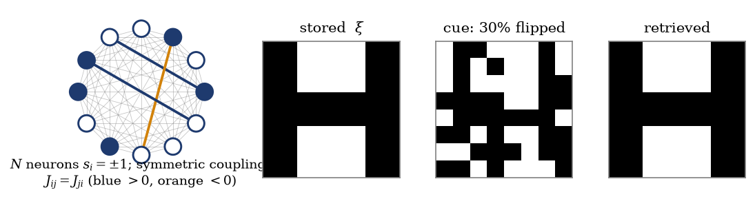
Figure 3.2 shows the machine in action before we prove anything about it: three \(8\times 8\) patterns stored in a network of \(N = 64\) neurons, one of them corrupted by flipping \(30\%\) of its pixels, and the corrupted cue handed to the dynamics Equation 3.1. The network repairs it completely.
Figure 3.2: A Hopfield network doing its job. Left: the model — \(N\) fully connected binary neurons \(s_i = \pm 1\) with symmetric couplings \(J_{ij}\) (spin = neuron, coupling = weight, local field = pre-activation). Right: one of three stored \(8 \times 8\) patterns (\(N = 64\), \(P = 3\)); the same pattern with \(30\%\) of its pixels flipped (overlap \(m_0 \approx 0.41\)); and the fixed point reached by the asynchronous dynamics Equation 3.1 — the memory, recovered exactly (\(m = 1\)).
3.4 The energy never increases
We owe the landscape cartoon a theorem. For continuous variables, “downhill” means gradient flow and \(\dot{E} \le 0\); for discrete spins there is no gradient, so what, precisely, guarantees descent? The derivation is short.
Let neuron \(k\) update by Equation 3.1: \(s_k \to s_k' = \operatorname{sign}(h_k)\), all other spins held fixed. In the energy Equation 3.2, collect the terms containing \(s_k\). The variable \(s_k\) appears twice in the double sum — once as \(i = k\) and once as \(j = k\) — and the symmetry\(J_{ij} = J_{ji}\) merges the two appearances into a single term:
where we used \(J_{kk} = 0\) so that the sum defining \(h_k\) is the full local field — and, crucially, \(h_k\)does not depend on \(s_k\) itself: it is the same number before and after the update. Since the spectator terms cancel in the difference, the energy change of the single update is exactly
\[
\Delta E \;=\; E' - E \;=\; -\,(s_k' - s_k)\, h_k.
\]
Two cases exhaust the possibilities. ① If \(s_k\) is already aligned with its field, \(s_k = \operatorname{sign}(h_k)\), the update does nothing: \(s_k' = s_k\) and \(\Delta E = 0\). ② If it is misaligned, the update flips it, \(s_k' = -s_k = \operatorname{sign}(h_k)\); then \(s_k' - s_k = 2 s_k'\) and \(s_k' h_k = |h_k|\), so
\[
\Delta E = -2\, |h_k| \;<\; 0.
\]
In both cases,
\[
\Delta E \le 0 \quad \text{under asynchronous updates with symmetric } J, \;\; J_{ii} = 0,
\tag{3.3}\]
Lyapunov property
with equality precisely when the chosen spin was already aligned.
Convergence follows at once. The energy is bounded below — crudely, \(E \ge -\frac{1}{2}\sum_{i \neq j} |J_{ij}|\) — and the configuration space is finite, so \(E\) takes finitely many values; every strict move lowers \(E\) by a positive amount, so no configuration can ever recur after a strict move. The dynamics must therefore reach, in finite time, a state from which no single-spin update changes anything: a fixed point, satisfying \(s_i = \operatorname{sign}(h_i)\) for every \(i\) — a local minimum of \(E\) against all single flips.
⇒ The cartoon is now a theorem: the network state flows monotonically downhill on \(E\) and halts at a local minimum. \(E\) is a Lyapunov function for the dynamics — the dynamicist’s certificate that a system computes something definite. If we can place the minima, we have built a content-addressable memory.
Both assumptions are essential. Symmetry is what made the energy’s \(s_k\)-terms collapse onto the same \(h_k\) that the update rule consults — with asymmetric couplings, the quantity the update aligns with and the quantity the energy penalizes are different objects, no energy function exists at all, and the dynamics is free to cycle or wander chaotically. Asynchrony ensured that only one term changes at a time; the synchronous variant — all spins updated in parallel, which is Little’s model (Little 1974) — loses the guarantee and admits stable period-2 oscillations, in which two configurations toss the network back and forth forever. And \(J_{ii} = 0\) is not cosmetic either: a self-coupling would put a \(J_{ii} s_i\) term into the field \(h_i = \sum_j J_{ij} s_j\) that spin \(i\) consults, biasing the spin toward its own current value — the update would then depend on \(s_i\) itself, breaking the very alignment of field and energy gradient that the descent argument above relied on. In the extreme of strong positive \(J_{ii}\), every configuration freezes into a fixed point — which is to say, no memory at all.
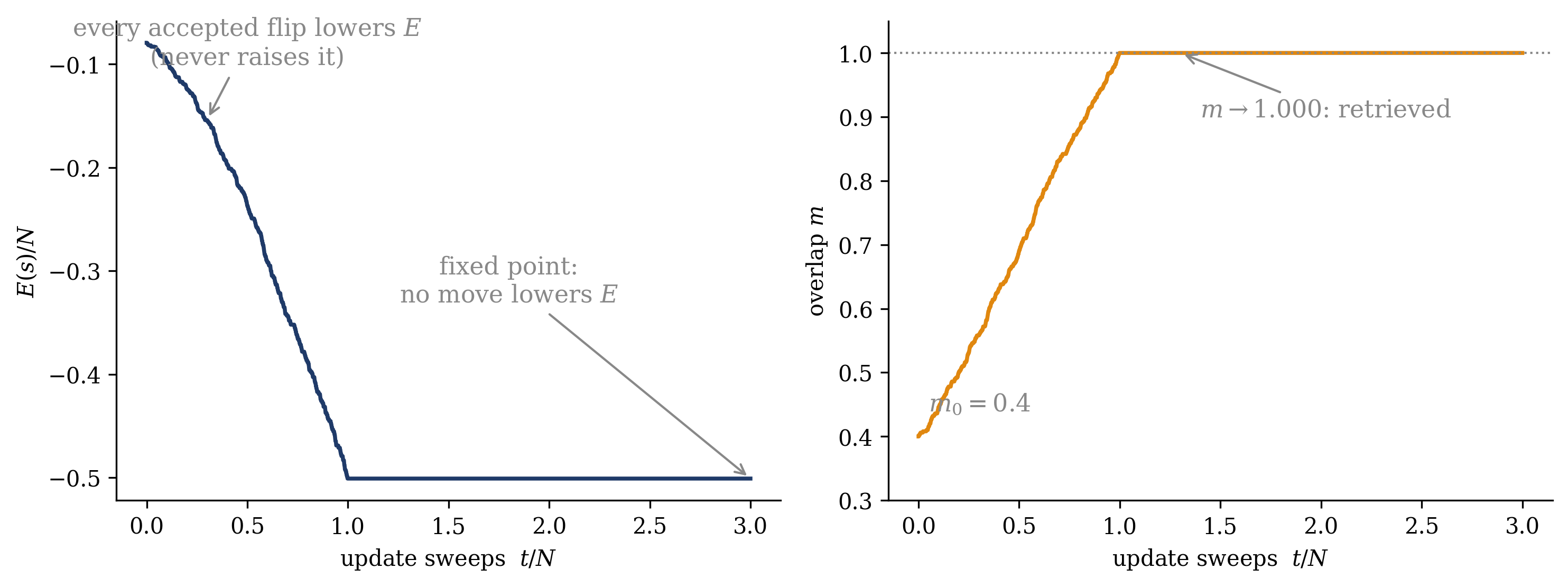
Figure 3.3 shows the theorem at work on a real network — \(N = 1000\) neurons, twenty stored patterns, a cue with \(30\%\) of its bits flipped: the energy descends as a monotone staircase, one small drop per accepted flip, and locks onto a plateau within a single sweep while the overlap with the stored pattern climbs to one.
Show code
rng = np.random.default_rng(2)N, P =1000, 20X = rng.choice([-1.0, 1.0], size=(P, N)) # P random patternsJ = (X.T @ X) / N; np.fill_diagonal(J, 0.0) # Hebb couplings, no self-couplings = X[0].copy()flip = rng.choice(N, size=int(0.30* N), replace=False) # 30% corrupted -> m0 = 0.4s[flip] *=-1E =-0.5* s @ (J @ s); xi0 = X[0]Es, ms = [E / N], [xi0 @ s / N]for k in np.concatenate([rng.permutation(N) for _ inrange(3)]): # 3 asynchronous sweeps h = J[k] @ s sk = np.sign(h) or1.0if sk != s[k]: E +=-(sk - s[k]) * h # exact single-flip energy change s[k] = sk Es.append(E / N); ms.append(xi0 @ s / N)t = np.arange(len(Es)) / Nfig, (a1, a2) = plt.subplots(1, 2, figsize=(10.0, 3.8))a1.plot(t, Es, color=NAVY, lw=1.8)a1.annotate("every accepted flip lowers $E$\n(never raises it)", xy=(0.3, Es[300]), xytext=(0.5, -0.1), color=GRAY, fontsize=11, ha="center", arrowprops=dict(arrowstyle="->", color=GRAY, lw=1))a1.annotate("fixed point:\nno move lowers $E$", xy=(3.0, Es[-1]), xytext=(1.8, -0.33), color=GRAY, fontsize=11, ha="center", arrowprops=dict(arrowstyle="->", color=GRAY, lw=1))a1.set_xlabel(r"update sweeps $t/N$"); a1.set_ylabel(r"$E(s)/N$")a2.plot(t, ms, color=ORANGE, lw=1.8)a2.axhline(1.0, color=GRAY, ls=":", lw=1)a2.annotate(r"$m\to 1.000$: retrieved", xy=(1.3, 1.0), xytext=(1.4, 0.9), color=GRAY, fontsize=11, arrowprops=dict(arrowstyle="->", color=GRAY, lw=1))a2.text(0.05, 0.44, r"$m_0=0.4$", color=GRAY, fontsize=11)a2.set_xlabel(r"update sweeps $t/N$"); a2.set_ylabel(r"overlap $m$"); a2.set_ylim(0.3, 1.05)fig.tight_layout(); plt.show()
Figure 3.3: The Lyapunov theorem at work: a Hopfield network with \(N = 1000\) neurons and \(P = 20\) stored patterns (\(\alpha = 0.02\)), cued with a stored pattern corrupted in \(30\%\) of its bits (\(m_0 = 0.4\)). Left: the energy per neuron under asynchronous updates — a monotone staircase, \(\Delta E \le 0\) at every single step, reaching a fixed point within one sweep (here \(E/N \to -0.50\)). Right: the overlap \(m\) with the cued memory climbing from \(0.4\) to \(1.000\) — exact retrieval.
Trap
Symmetry and asynchrony are load-bearing, not stylistic. Drop symmetry and no energy function exists — the dynamics can cycle or run chaotically. Keep symmetry but update synchronously and period-2 limit cycles survive. The energy-landscape picture of neural computation rests on these two assumptions — and note the scope: real cortical synapses are asymmetric, so biology sits outside the theorem.
3.5 Hebbian storage
The theorem guarantees arrival at a minimum; we now place the minima. Given \(P\) patterns \(\xi^\mu \in \{-1, +1\}^N\), \(\mu = 1, \dots, P\) — the memories, drawn for the theory below as independent unbiased random signs — choose the couplings as a sum of outer products:
This is Hebb’s postulate (Hebb 1949) — neurons that fire together, wire together — written as an equation: every pair of units that agrees in a pattern has its coupling strengthened, every pair that disagrees has it weakened, pattern by pattern, with the \(1/N\) holding the local fields at order one. The rule is symmetric by construction, so the theorem of Section 3.4 applies without further work. In machine-learning terms it is one-shot learning: the weights are read off the data in a single pass, with no loss function to descend and no iteration. Week 3 replaces this fiat with gradient descent on a likelihood, and it is in that gradient that \(Z\) reappears.
Does it work? One pattern, verified. Store a single pattern (\(P = 1\)) and evaluate the local field at the pattern itself, \(s = \xi\):
Every spin sits aligned with its field, with a uniform stability margin of order one: \(\xi\) is a fixed point of Equation 3.1, hence by Section 3.4 a local minimum of the energy. (So, immediately, is the flipped pattern \(-\xi\): the energy Equation 3.2 is even under a global flip \(s \to -s\) — our first minimum that nobody ordered. We collect the others below.)
More is true, and it introduces the week’s order parameter. Define the overlap of the network state with a pattern,
which counts agreement: \(m = 1\) is perfect retrieval, \(m = 0\) is chance, and \(m_0 = 1 - 2f\) for a cue corrupted in a random fraction \(f\) of its bits. For \(P = 1\) the local field at any state collapses onto the overlap,
so a single sweep of Equation 3.1 sets every spin to \(\operatorname{sign}(\xi_i m) = \xi_i\) whenever \(m > 0\): any cue with positive initial overlap retrieves the memory in one sweep, and the basin of \(\xi\) is the entire \(m > 0\) half of the hypercube — \(2^{N-1}\) configurations — with the mirror image \(-\xi\) owning the other half. You have seen this \(m\) before: it is exactly the magnetization that indexed the free-energy saddle of Section 2.5, now reinterpreted as how retrieved a memory is. The order-parameter language of Week 1 carries over directly, and the next lecture makes quantitative use of it.
Many patterns: signal and crosstalk. With \(P\) patterns stored, evaluate the aligned local field at one of them, \(s = \xi^\mu\), splitting the Hebb sum into the term \(\nu = \mu\) and the rest:
The stored pattern contributes a clean unit signal — that is the \(P = 1\) calculation again. Everything else contributes crosstalk: a sum of \((P-1)(N-1)\) terms, each \(\pm 1/N\) with a pseudo-random sign, since the patterns are independent. By the central limit theorem, \(C_i\) is approximately Gaussian with mean zero and variance
where \(\alpha\) is the storage load, the number of patterns per neuron. The entire question of memory capacity is now visible in one line: a bit of the stored pattern is stable as long as its signal beats its noise, and the competition is between \(1\) and a Gaussian of width \(\sqrt{\alpha}\). How that competition ends, and why it ends abruptly rather than gradually, is the next lecture; the example below is the first look at the numbers.
Take-home 2
The Hebb rule \(J_{ij} = \frac{1}{N} \sum_\mu \xi_i^\mu \xi_j^\mu\) writes the memories directly into the couplings — learning in one shot, no gradient. Each stored pattern feels a unit signal plus Gaussian crosstalk of width \(\sqrt{P/N}\) from all the others: memory works until the stored patterns start to interfere.
3.6 Example: retrieval, then interference
Retrieval from heavy corruption (\(P = 1\)). Store one pattern in \(N = 1000\) neurons and corrupt it heavily: flip a random \(40\%\) of the bits, leaving the initial overlap \(m_0 = 1 - 2 \times 0.4 = 0.2\). By the field formula of Section 3.5, every neuron feels \(h_i \approx 0.2\, \xi_i\) — a weak field, but pointing the right way at every single site, because with one pattern there is no noise to point it wrong. One asynchronous sweep restores \(m = 1\) exactly. Running the actual dynamics confirms the table:
The stored pattern sits at energy \(E(\xi)/N = -(N-1)/2N \approx -1/2\) per neuron — extensively deep. The lesson of the table calibrates what comes next: with a single stored pattern, retrieval is robust — the basin is half of configuration space — so the dynamics is never what limits an associative memory; interference is.
Interference: the first-sweep error rate. Now store \(P\) patterns and read the aligned field on one of them: signal \(1\), Gaussian crosstalk of width \(\sqrt{\alpha}\). A bit comes out wrong on the first sweep when the crosstalk overwhelms its signal, \(C_i < -1\), which happens with probability
The Gaussian tail sweeps this quantity across twenty orders of magnitude over the loads in the table:
\(\alpha = P/N\)
\(P\) at \(N = 1000\)
\(P_\text{err}\)
wrong bits per retrieved pattern
reading
\(0.01\)
\(10\)
\(\sim 10^{-23}\)
\(0\)
interference invisible
\(0.05\)
\(50\)
\(4 \times 10^{-6}\)
\(0.004\)
still essentially perfect
\(0.10\)
\(100\)
\(8 \times 10^{-4}\)
\(0.8\)
first wrong bits — and errors feed back
\(0.138\)
\(138\)
\(3.6 \times 10^{-3}\)
\(3.6\)
the edge (why here? — next lecture)
\(0.20\)
\(200\)
\(1.3 \times 10^{-2}\)
\(13\)
avalanche territory
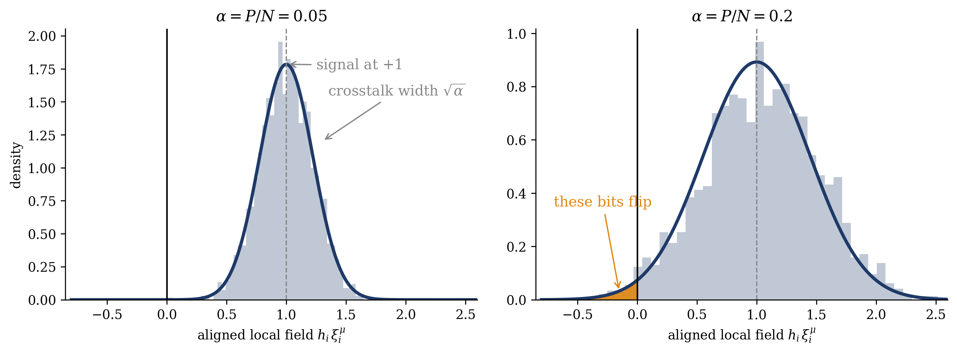
Figure 3.4 shows the same story measured rather than estimated: the empirical distribution of the aligned local field across the sites of a stored pattern, in a network of \(N = 2000\) neurons, at two loads. At \(\alpha = 0.05\) the Gaussian sits comfortably to the right of zero and, in the simulation, not one of the \(2000\) bits is unstable. At \(\alpha = 0.2\) a visible tail has leaked past zero — \(1.6\%\) of bits in this realization, against the Gaussian estimate of \(1.3\%\) — and each of those bits, once flipped, adds noise to the fields of all the others.
That feedback is what the table leaves out. The erfc column is a first-sweep, no-feedback estimate; it does not by itself locate the storage limit. Flipped bits degrade the fields, which flip more bits — and whether the avalanche self-limits or runs away is a self-consistency question, not a one-line Gaussian one. Its answer is one of the celebrated results of the field: retrieval survives up to a sharp critical load \(\alpha_c \approx 0.138\) and then collapses discontinuously — memory dies as a phase transition, not a fade (Amit, Gutfreund, and Sompolinsky 1985, 1987). The next lecture builds the self-consistent argument; in the tutorial you will cross \(\alpha_c\) yourself and watch it happen. (For calibration: Hopfield (1982) already reported, numerically, that recall degrades severely beyond \(P \approx 0.15\, N\) — close to the sharp answer computed three years later.)
Figure 3.4: Signal versus crosstalk, measured. Histograms of the aligned local field \(h_i \xi_i^\mu\) over the \(N = 2000\) sites of a stored pattern, with the Gaussian \(\mathcal{N}(1, \alpha)\) overlaid. Left, load \(\alpha = P/N = 0.05\): the crosstalk is narrow, the entire distribution sits right of zero, and no bit is unstable. Right, \(\alpha = 0.2\): the width \(\sqrt{\alpha}\) has grown until a tail (shaded) leaks past zero — those bits flip on the first sweep (\(1.6\%\) measured here versus \(1.3\%\) from the Gaussian estimate), and their errors feed back into every other field. Where this avalanche becomes fatal is the next lecture’s calculation.
Energy stops being something we measure and becomes something we design. That is the banner of Module 1 — and everything that follows in this course, through the Boltzmann machine to the diffusion model, inherits it.
One practical pointer, because this week’s tutorial is built on exactly this material: the warm-up card (due the evening before the next lecture) works from this lecture and from Hopfield (1982), and it primes the field decomposition above — signal against crosstalk. The hard problem in the tutorial builds on it.
Take-home 3
One stored pattern owns half of configuration space, so dynamics never limits an associative memory — interference does. Capacity is a competition between a unit signal and crosstalk of width \(\sqrt{P/N}\): quantified in the next lecture, experienced in the tutorial.
3.7 What the landscape contains besides your data
The landscape contains more minima than we stored, and the extras matter for what follows.
Three families of uninvited minima populate the landscape. ① The flipped patterns\(-\xi^\mu\), exactly degenerate with the originals by the global symmetry \(s \to -s\) of Equation 3.2 — harmless in practice (fix one bit’s meaning and the ambiguity is gone) but a genuine doubling of the attractor count. ② Mixture states: symmetric blends of odd numbers of patterns, the simplest being the three-pattern majority \(s_i = \operatorname{sign}(\xi_i^1 + \xi_i^2 + \xi_i^3)\), which for random patterns has overlap \(1/2\) with each of its three parents and is a genuine local minimum — the network’s version of a confused recollection that merges three memories. ③ At larger loads, spin-glass states: minima essentially uncorrelated with anything stored, the rugged debris of the crosstalk. The lesson: a designed landscape is still a landscape — you specify the minima you want, and the geometry supplies others for free. There is even a first argument here for Week 3’s turn to finite temperature: the spurious minima are typically shallower than the retrieval states, so a little thermal noise destabilizes them before the memories — the same temperature that brings back \(Z\) and the Boltzmann distribution also cleans the landscape.
A biological disclaimer is in order, since the model uses the word “neuron.” Real synapses are not symmetric; real neurons are not binary; real updates are not asynchronous-random; and Hopfield (1984) himself showed the collective behavior survives at least the second idealization, in a graded-response (continuous) variant we merely name. The model’s value is not fidelity to cortex — it is that it is minimal, solvable, and generalizable: the energy-based and diffusion models of the rest of the course inherit its shape, which is exactly the sense in which the 2024 Nobel citation calls it foundational.
Trap
Convergence is not correctness. The Lyapunov theorem guarantees arrival at some minimum; whether it is the cued memory, its mirror image, or a mixture is a question about basin geometry, which the theorem does not touch. And do not invert Take-home 1: “stored patterns are minima” is true; “minima are stored patterns” is false.
3.8 Outlook
The next lecture takes the question this lecture left open — how many patterns fit? — and answers it quantitatively: the signal-to-noise argument made self-consistent, the error avalanche tamed or not, the strict-stability estimate \(P_\text{max} \approx N / (2 \ln N)\) for perfect recall of every bit, and the celebrated retrieval boundary \(\alpha_c \approx 0.138\) of Amit, Gutfreund, and Sompolinsky (1985) — with the caveat that the full derivation runs on replica machinery this course quotes rather than builds; Module 2 acquires its modern mean-field descendants, and the free-energy saddle of Section 2.5 returns there in earnest. In the tutorial, you will load a network past \(\alpha_c\) and watch memory die as a phase transition.
Then Week 3 brings back the partition function. Today’s network was deterministic and stored its patterns by fiat. Do the two natural next things — heat it up, so that the update rule becomes stochastic and the stationary law becomes exactly Week 1’s Boltzmann distribution over the designed energy; and ask it to learn\(J\) by maximum likelihood rather than by Hebb’s fiat — and the training gradient acquires a term \(\nabla_{\!J} \log Z\). That term is intractable, it is the negative phase of the Boltzmann machine, and it is the central obstruction of energy-based learning. The energy landscape was designed today; from Week 3 on, training it requires computing \(Z\).
Amit, Daniel J. 1989. Modeling Brain Function: The World of Attractor Neural Networks. Cambridge: Cambridge University Press.
Amit, Daniel J., Hanoch Gutfreund, and Haim Sompolinsky. 1985. “Storing Infinite Numbers of Patterns in a Spin-Glass Model of Neural Networks.”Physical Review Letters 55 (14): 1530–33. https://doi.org/10.1103/PhysRevLett.55.1530.
Edwards, Samuel F., and Philip W. Anderson. 1975. “Theory of Spin Glasses.”Journal of Physics F: Metal Physics 5 (5): 965–74. https://doi.org/10.1088/0305-4608/5/5/017.
Hebb, Donald O. 1949. The Organization of Behavior: A Neuropsychological Theory. New York: Wiley.
Hertz, John, Anders Krogh, and Richard G. Palmer. 1991. Introduction to the Theory of Neural Computation. Redwood City: Addison-Wesley.
Hopfield, John J. 1982. “Neural Networks and Physical Systems with Emergent Collective Computational Abilities.”Proceedings of the National Academy of Sciences 79 (8): 2554–58. https://doi.org/10.1073/pnas.79.8.2554.
———. 1984. “Neurons with Graded Response Have Collective Computational Properties Like Those of Two-State Neurons.”Proceedings of the National Academy of Sciences 81 (10): 3088–92. https://doi.org/10.1073/pnas.81.10.3088.
MacKay, David J. C. 2003. Information Theory, Inference, and Learning Algorithms. Cambridge: Cambridge University Press.
McCulloch, Warren S., and Walter Pitts. 1943. “A Logical Calculus of the Ideas Immanent in Nervous Activity.”Bulletin of Mathematical Biophysics 5: 115–33. https://doi.org/10.1007/BF02478259.
Mehta, Pankaj, Marin Bukov, Ching-Hao Wang, Alexandre G. R. Day, Clint Richardson, Charles K. Fisher, and David J. Schwab. 2019. “A High-Bias, Low-Variance Introduction to Machine Learning for Physicists.”Physics Reports 810: 1–124. https://doi.org/10.1016/j.physrep.2019.03.001.
Nishimori, Hidetoshi. 2001. Statistical Physics of Spin Glasses and Information Processing: An Introduction. Oxford: Oxford University Press.