4 Storage capacity: how memory dies – From Boltzmann to Diffusion

4.1 Is \(0.15\,N\) the answer?

We start from where the last lecture left us, in three lines. We design the energy: Hebb’s rule Equation 3.4 writes \(P\) patterns into the couplings in one shot. Descent is a theorem: for symmetric couplings and asynchronous updates, the dynamics rolls monotonically downhill and halts in a local minimum (Section 3.4). And at a stored pattern, every neuron’s aligned local field splits as

\[ h_i\, \xi_i^\mu \;=\; 1 \;+\; C_i , \]

a clean unit signal plus a crosstalk term \(C_i\) that we named and deliberately did not compute (Section 3.5). What remains is the computation of \(C_i\) — and of what the network does about it.

There is also a number on the table, and it came from your own reading. Hopfield (1982) reports, from simulations of networks of \(N = 100\) neurons, that recall degrades severely once the number of stored patterns exceeds about \(0.15\,N\). The obvious question is: is \(0.15\) the answer? It cannot be accepted as it stands, for two reasons that turn out to carry real physics. First, we do not yet know which question it answers. “How many patterns fit?” splits, on inspection, into two demands with no obligation to agree: strict stability — every bit of every stored pattern sits aligned with its field, no exceptions, so the memories are exact fixed points — and retrieval — the pattern is recalled up to a small dressing of wrong bits, and cues in its basin still flow to it. The first is a worst-case demand, governed by the largest of \(NP\) random crosstalk pulls; the second is a typical-case demand, governed by the bulk of the crosstalk distribution. You have met this split before in other fields: worst-case versus average-case in the analysis of algorithms, minimum-distance versus Shannon capacity in coding theory (MacKay 2003). The two answers here differ not by a constant but by a factor of \(\ln N\).

Second, we do not know how memory fails when it fails. The natural guess — more patterns, gradually more wrong bits, memory dimming like an old photograph — is wrong, and wrong in an instructive way. The truth is a cliff: retrieval survives, nearly intact, up to a sharp critical load, and then collapses discontinuously. Understanding why it is a cliff is the substance of the analysis below — the course’s first genuine phase transition, found inside a learning machine rather than a magnet.

Today we compute what interference costs, and find that the answer depends on what we demand — perfection is sublinear, tolerance is extensive — and that when Hebbian memory fails, it fails all at once.

The partition function stays out of sight: everything until the final section happens at \(T = 0\). The difficulty is interference, and the tool that quantifies it is the central limit theorem. The lecture also does to Hopfield’s model what Amit, Gutfreund, and Sompolinsky (1985) did — computes its phase diagram. The diagram has a temperature axis, and the final section explains why Week 3 walks up that axis on purpose.

Take-home 1

“How many patterns fit?” is two questions. Demanding every stored bit be exactly stable gives \(P_\text{max} \approx N / (2 \ln N)\) — perfection costs a logarithm. Tolerating a percent of wrong bits gives extensive capacity \(P_\text{max} = \alpha_c N\) with \(\alpha_c \approx 0.138\). Capacity is not a property of the network alone; it is a property of the network plus the demand placed on it.

4.2 The statistics of interference

The first task is the distribution of the crosstalk. Recall its definition — at stored pattern \(\xi^\mu\), the aligned field on site \(i\) carries, besides the unit signal,

\[ C_i \;=\; \frac{1}{N} \sum_{\nu \neq \mu} \sum_{j \neq i} \xi_i^\mu\, \xi_i^\nu\, \xi_j^\nu\, \xi_j^\mu \;\equiv\; \frac{1}{N} \sum_{\nu \neq \mu} \sum_{j \neq i} t_{\nu j}, \]

a sum of \((P-1)(N-1)\) terms \(t_{\nu j} = \pm 1\), each a product of four independent, unbiased signs. The bookkeeping takes one careful paragraph, because “pseudo-random” needs justification. Each term has mean zero: for \(\nu \neq \mu\) and \(j \neq i\) the four factors involve at least one sign that appears exactly once, and its average kills the product. Better, the terms are pairwise uncorrelated: for two distinct index pairs \((\nu, j) \neq (\nu', j')\), the expectation \(\langle t_{\nu j}\, t_{\nu' j'} \rangle\) always contains some pattern entry to an odd power — if \(\nu \neq \nu'\) the two patterns are independent and each factor averages to zero separately; if \(\nu = \nu'\) but \(j \neq j'\) the product contains \(\xi_j^\mu \xi_{j'}^\mu\) times signs of pattern \(\nu \ne \mu\), and again averages to zero. So the variance of the sum is exactly the sum of the variances — no approximation yet:

\[ \operatorname{Var}(C_i) \;=\; \frac{(P-1)(N-1)}{N^2} \;\approx\; \frac{P}{N} \;=\; \alpha . \]

(Full independence does fail at higher orders — quadruples of terms can share signs — but these correlations affect the distribution only at relative order \(1/N\).) The central limit theorem then does the rest: for large \(N\) at fixed load \(\alpha\),

\[ C_i \;\sim\; \mathcal{N}(0,\, \alpha), \qquad \alpha = \frac{P}{N}. \tag{4.1}\]

crosstalk statistics

The physical reading: the signal is \(1\) no matter how many patterns are stored; the noise grows as \(\sqrt{P/N}\) — and interference depends on \(P\) and \(N\) only through their ratio. The load \(\alpha\) is the model’s control parameter, and all quantities below are functions of it.

A stored bit comes out wrong on the first update sweep when the crosstalk overwhelms its signal, \(1 + C_i < 0\) — a fluctuation of \(1/\sqrt{\alpha}\) standard deviations. The Gaussian tail integral (the Gaussian integral of Section 2.4, at work once more) gives the first-sweep bit-error probability you already met empirically in Section 3.6:

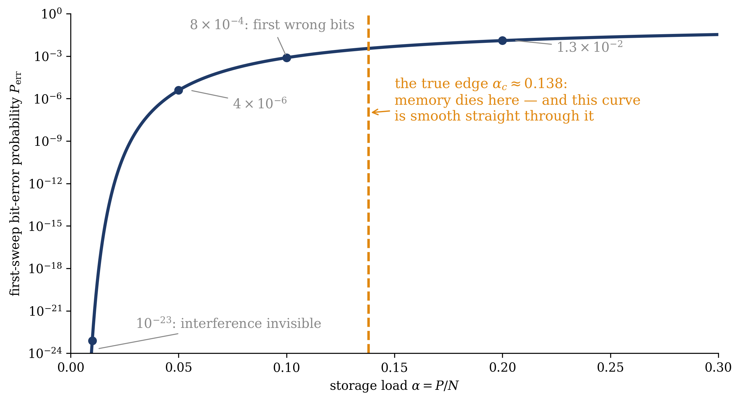
\[ P_\text{err} \;=\; \Pr[\,C_i < -1\,] \;=\; \tfrac{1}{2} \operatorname{erfc}\!\Big( \frac{1}{\sqrt{2\alpha}} \Big). \tag{4.2}\]

first-sweep error rate

Figure 4.1 plots it, and the plot teaches two things at once. The first is the steepness of a Gaussian tail: between \(\alpha = 0.01\) and \(\alpha = 0.2\) — a factor of twenty in load — the error probability climbs by twenty-one orders of magnitude, from \(10^{-23}\) to \(10^{-2}\). Steepness like this is why the capacity question has a sharp answer at all: whatever criterion we impose, the crossover from “satisfied absurdly well” to “violated badly” is compressed into a narrow window of \(\alpha\). The second lesson is a warning, drawn on the figure deliberately: the curve is perfectly smooth through \(\alpha_c \approx 0.138\), the load where memory actually dies. Nothing in the first-sweep error rate marks the edge; that mismatch is the central puzzle of the analysis.

Show code

fig, ax = plt.subplots(figsize=(8.4, 4.6))
al = np.linspace(0.004, 0.30, 500)
Perr = 0.5 * erfc(1 / np.sqrt(2 * al))
ax.semilogy(al, Perr, color=NAVY, lw=2.5)
ax.axvline(0.138, color=ORANGE, ls="--", lw=2)
labels = {0.01: r"$10^{-23}$: interference invisible", 0.05: r"$4\times 10^{-6}$",
          0.10: r"$8\times 10^{-4}$: first wrong bits", 0.20: r"$1.3\times 10^{-2}$"}
for a in labels:
    ax.plot([a], [0.5 * erfc(1 / np.sqrt(2 * a))], "o", color=NAVY, ms=6)
for a, xy, xt in [(0.01, (0.012, 2e-24), (0.03, 6e-23)), (0.05, (0.055, 4e-6), (0.075, 2e-7)),
                  (0.10, (0.10, 9e-4), (0.055, 8e-2)), (0.20, (0.205, 1.3e-2), (0.225, 2e-3))]:
    ax.annotate(labels[a], xy=xy, xytext=xt, color=GRAY, fontsize=10.5,
                arrowprops=dict(arrowstyle="-", color=GRAY, lw=0.8))
ax.annotate("the true edge $\\alpha_c\\approx 0.138$:\nmemory dies here — and this curve\n"
            "is smooth straight through it", xy=(0.138, 1e-7), xytext=(0.15, 3e-8),
            color=ORANGE, fontsize=11, ha="left",
            arrowprops=dict(arrowstyle="->", color=ORANGE, lw=1))
ax.set_xlabel(r"storage load $\alpha = P/N$")
ax.set_ylabel(r"first-sweep bit-error probability $P_\mathrm{err}$")
ax.set_ylim(1e-24, 1); ax.set_xlim(0, 0.30)
fig.tight_layout(); plt.show()

Figure 4.1: The first-sweep bit-error probability \(P_\text{err} = \frac{1}{2}\operatorname{erfc}(1/\sqrt{2\alpha})\) of Equation 4.2, on a logarithmic scale. The Gaussian tail is remarkably steep — twenty-one orders of magnitude between \(\alpha = 0.01\) and \(\alpha = 0.2\) — which is why capacity questions have sharp answers. But note the dashed line: the true storage limit \(\alpha_c \approx 0.138\), where retrieval collapses, leaves no trace whatsoever on this curve. First-sweep error rates cannot locate the transition; the transition is made of feedback.

4.3 Perfection costs a logarithm

Now impose the strong demand: strict stability. Every stored pattern should be an exact fixed point of the dynamics — all \(N\) bits of all \(P\) patterns aligned with their fields, so that a memory, once retrieved, is letter-perfect. How many patterns does that permit?

Consider first a single stored pattern and ask that all \(N\) of its bits hold. Bit failures are (to leading order) independent rare events with probability \(P_\text{err}\) each, so the expected number of unstable bits is \(N P_\text{err}\), and the pattern is exactly stable, with high probability, as long as

\[ N\, P_\text{err} \;\lesssim\; 1 . \]

Insert the Gaussian tail asymptotic — for \(x \gg 1\), \(\tfrac12\operatorname{erfc}(x/\sqrt{2}) \approx e^{-x^2/2} / (x \sqrt{2\pi})\), here with \(x = 1/\sqrt{\alpha}\) — and keep only the exponentially dominant balance:

\[ N \sqrt{\frac{\alpha}{2\pi}}\; e^{-1/2\alpha} \;\approx\; 1 \qquad \Longrightarrow \qquad \frac{1}{2\alpha} \;\approx\; \ln N + \mathcal{O}(\ln \ln N), \]

where the prefactor’s logarithm is subleading and swept into the correction. Solving for the load,

\[ \boxed{\; \alpha_\text{strict} \approx \frac{1}{2 \ln N}, \qquad P_\text{max} \approx \frac{N}{2 \ln N} \;} \tag{4.3}\]

strict-stability capacity

— sublinear in \(N\). If instead we demand that every pattern be letter-perfect simultaneously, the union runs over all \(NP \approx \alpha N^2\) bits, the balance becomes \(\frac{1}{2\alpha} \approx \ln(N P) \approx 2 \ln N\), and the capacity halves again to \(P_\text{max} \approx N/(4 \ln N)\). Both statements — with the constants, the basin-of-attraction refinements, and full rigor in place of our union-bound physics — are the content of a celebrated information-theory paper (McEliece et al. 1987); our two-line estimate lands exactly on their scalings.

⇒ Demanding zero errors makes capacity sublinear: the price of perfection is a logarithm, and the logarithm counts how many trials you insist survive. The mechanism recurs across physics and statistics: the maximum of \(M\) independent Gaussian pulls grows like \(\sqrt{2 \ln M}\), so the worst bit in the network — not the typical one — sets the rule, and worst cases cost logarithms. At \(N = 1000\): about \(72\) patterns (\(36\) if every pattern must be perfect). Hopfield’s \(150\) is nowhere in sight — so either his simulations were wrong, or exact fixed points are the wrong demand. They were not wrong.

Notice what strict stability does not say. A pattern that fails it has, at \(\alpha = 0.1\), roughly one misaligned bit per thousand: the dynamics flips that bit, the state comes to rest one or two spin flips away from the stored pattern, and any user of the memory would call the recall a success. Strict stability is a bookkeeping demand, not a statement about whether the memory works. The working question — does a fixed point near \(\xi^\mu\) survive, with a basin around it? — is a question about the typical crosstalk and about what the first few errors do next. That question has more physics in it.

Trap

A small error rate is not safety. \(P_\text{err} = 10^{-4}\) sounds negligible, but there are \(NP\) stored bits: rare events at a fixed rate become certainties at scale, which is why the strict criterion collapses from “essentially never fails” to “fails somewhere, always” over a narrow range of \(\alpha\). Extreme-value reasoning — the worst of many — obeys different arithmetic than typical-value reasoning. Know which question you are asking.

4.4 The collapse

So relax the demand and follow the dynamics. Start the network at a stored pattern with a few wrong bits — or far from it, at overlap \(m\) — and ask what one sweep of updates does. For a state with overlap \(m\) with pattern \(\xi^\mu\) and no other special correlations, the same central-limit argument as before gives an aligned field \(m + \mathcal{N}(0, \alpha)\) on every site, so the overlap after one parallel sweep is the probability of ending aligned minus the probability of ending misaligned:

\[ m_1 \;=\; \operatorname{erf}\!\Big( \frac{m_0}{\sqrt{2\alpha}} \Big). \tag{4.4}\]

first-sweep retrieval map — legitimate once

This formula is valid for the first sweep only — a restriction that is about to matter. As a first-sweep statement it is already useful: it reproduces Equation 4.2 at \(m_0 = 1\) (since \(m_1 = 1 - 2P_\text{err}\)), and at small \(\alpha\) it becomes a step function of \(m_0\), recovering the one-pattern result of Section 3.5 that any positive initial overlap retrieves in a single sweep.

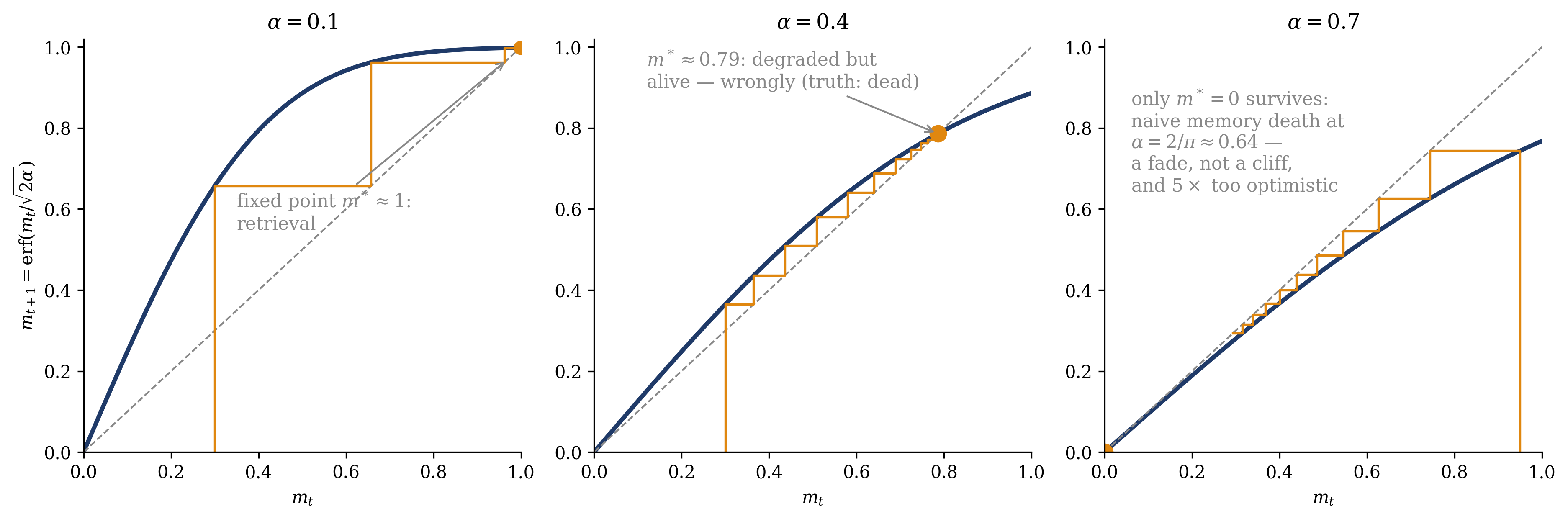
The natural next step is to iterate the map, treating each sweep as a fresh draw of Gaussian noise. Figure 4.2 cobwebs the map. The retrieval fixed point \(m^* = \operatorname{erf}(m^*/\sqrt{2\alpha})\) sits near \(1\) at small load, slides gracefully downward as \(\alpha\) grows, and survives — check the slope at the origin — all the way to \(\alpha = 2/\pi \approx 0.64\), where it vanishes continuously. The naive theory thus predicts that memory fades, with the overlap degrading smoothly and useful recall extending out to \(\alpha \approx 0.64\).

Both the number and the kind are wrong. The truth is \(\alpha_c \approx 0.138\) — five times smaller — and the failure is discontinuous. The calculation was clean and yet wrong by a factor of five: what did we throw away?

Show code

def fixed_point(alpha):                              # nonzero retrieval fixed point
    m = 0.99
    for _ in range(500):
        m = erf(m / np.sqrt(2 * alpha))
    return m
fig, axes = plt.subplots(1, 3, figsize=(12.6, 4.2))
configs = [(0.1, 0.3, 7, "fixed point $m^*\\approx 1$:\nretrieval", "near1"),
           (0.4, 0.3, 10, "$m^*\\approx 0.79$: degraded but\nalive — wrongly (truth: dead)", "dot"),
           (0.7, 0.95, 10, "only $m^*=0$ survives:\nnaive memory death at\n"
            "$\\alpha=2/\\pi\\approx 0.64$ —\na fade, not a cliff,\nand $5\\times$ too optimistic", "zero")]
for ax, (alpha, m0, nst, note, kind) in zip(axes, configs):
    mm = np.linspace(0, 1, 300)
    ax.plot(mm, erf(mm / np.sqrt(2 * alpha)), color=NAVY, lw=2.5)     # the map
    ax.plot([0, 1], [0, 1], color=GRAY, ls="--", lw=1)               # diagonal
    x = m0; xs_, ys_ = [x], [0.0]
    for _ in range(nst):                                             # cobweb
        y = erf(x / np.sqrt(2 * alpha)); xs_ += [x, y]; ys_ += [y, y]; x = y
    ax.plot(xs_, ys_, color=ORANGE, lw=1.3)
    if kind == "dot":
        mstar = fixed_point(alpha); ax.plot([mstar], [mstar], "o", color=ORANGE, ms=9)
        ax.annotate(note, xy=(mstar, mstar), xytext=(0.12, 0.9), color=GRAY, fontsize=10.5,
                    arrowprops=dict(arrowstyle="->", color=GRAY, lw=1))
    elif kind == "zero":
        ax.plot([0], [0], "o", color=ORANGE, ms=9)
        ax.text(0.06, 0.9, note, color=GRAY, fontsize=10.5, va="top")
    else:
        ax.plot([fixed_point(alpha)], [fixed_point(alpha)], "o", color=ORANGE, ms=7)
        ax.annotate(note, xy=(0.97, 0.97), xytext=(0.35, 0.55), color=GRAY, fontsize=10.5,
                    arrowprops=dict(arrowstyle="->", color=GRAY, lw=1))
    ax.set_title(rf"$\alpha = {alpha}$", fontsize=12)
    ax.set_xlabel(r"$m_t$"); ax.set_xlim(0, 1); ax.set_ylim(0, 1.02)
axes[0].set_ylabel(r"$m_{t+1} = \mathrm{erf}(m_t/\sqrt{2\alpha})$")
fig.tight_layout(); plt.show()

Figure 4.2: The naive theory and its instructive failure. The first-sweep retrieval map \(m_{t+1} = \operatorname{erf}(m_t/\sqrt{2\alpha})\) of Equation 4.4, cobwebbed at three loads. Left, \(\alpha = 0.1\): rapid convergence to a retrieval fixed point near \(m^* = 1\). Center, \(\alpha = 0.4\): the naive fixed point survives at \(m^* \approx 0.79\) — although the true network is long dead here. Right, \(\alpha = 0.7\): past \(\alpha = 2/\pi \approx 0.64\) only \(m^* = 0\) remains, and the naive theory predicts memory *fading* continuously to nothing. Both the predicted capacity and the predicted kind of failure are wrong, because iterating the map re-randomizes the crosstalk each sweep — precisely what the network does not do.

We threw away the feedback. Iterating Equation 4.4 assumes the crosstalk is re-randomized at every sweep — that the noise a spin feels now is statistically independent of the errors made earlier. It is not. A bit that flipped did so because the crosstalk pushed it; the flipped bit is therefore correlated with the noise, and through the couplings it pollutes the fields of every other site in a way that does not average out. Errors amplify the very noise that produced them. The correct self-consistent treatment — set up by Amit, Gutfreund, and Sompolinsky (1985) and carried out in full in Amit, Gutfreund, and Sompolinsky (1987) — replaces the bare noise variance \(\alpha\) by an amplified one, and at zero temperature its equations read (stated here, derived with Module 2’s tools):

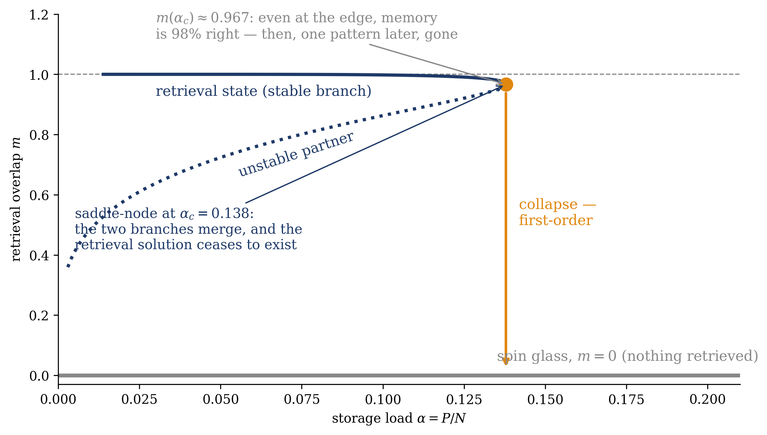
\[ m = \operatorname{erf}\!\Big( \frac{m}{\sqrt{2 \alpha r}} \Big), \qquad \chi = \sqrt{\frac{2}{\pi \alpha r}}\; e^{-m^2 / 2\alpha r}, \qquad r = \frac{1}{(1 - \chi)^2}, \tag{4.5}\]

AGS self-consistency at \(T=0\) (stated)

where \(\chi\) measures the network’s integrated response to its own errors — a susceptibility, distinct from the crosstalk \(C_i\) above — and \(r \ge 1\) is the factor by which that response inflates the crosstalk. Solving the three equations numerically — an afternoon’s exercise once you trust them, and Figure 4.3 is exactly that computation — produces the picture the naive map could not. As \(\alpha\) grows, the retrieval solution (overlap near one) is approached from below by an unstable partner solution; the two branches bend toward each other, meet, and annihilate at

\[ \boxed{\; \alpha_c \;\approx\; 0.138, \qquad m(\alpha_c) \approx 0.97. \;} \tag{4.6}\]

storage capacity (Amit–Gutfreund–Sompolinsky)

This is a saddle-node bifurcation: beyond \(\alpha_c\) the retrieval state does not degrade — it ceases to exist, and the dynamics has nowhere to fall but the spin-glass phase at \(m = 0\). The overlap jumps discontinuously from \(0.97\) to \(0\): memory death is a first-order transition. And the number \(0.97\) is itself the transition’s signature: even at the edge, retrieval is still \(98.4\%\) correct per bit. Memory near capacity remains nearly perfect — and then, one pattern later, it is absent. (For the physics-native: a discontinuous order parameter with no symmetry broken between the phases — the transition is about a metastable branch existing or not, spinodal-flavored rather than Ising-flavored. Module 2 gives this remark its proper home.)

Show code

def branch(yv):                                      # AGS T=0 solution, parametrized by y
    m = erf(yv)
    chi = (2 * yv * np.exp(-yv**2)) / (np.sqrt(np.pi) * m)   # AGS susceptibility χ
    alpha = m**2 * (1 - chi)**2 / (2 * yv**2)
    return alpha, m
a_st, m_st = branch(np.linspace(1.5, 6, 400))        # stable branch  (y > y_fold)
a_un, m_un = branch(np.linspace(0.33, 1.5, 400))     # unstable branch (y < y_fold)
ac, mc = branch(np.array([1.5])); ac, mc = ac[0], mc[0]   # the fold
fig, ax = plt.subplots(figsize=(8.6, 4.8))
ax.axhline(1.0, color=GRAY, ls="--", lw=0.9); ax.axhline(0.0, color=GRAY, lw=3)
ax.plot(a_st, m_st, color=NAVY, lw=2.5)
ax.plot(a_un, m_un, color=NAVY, ls=":", lw=2.5)
ax.plot([ac], [mc], "o", color=ORANGE, ms=10)
ax.annotate("", xy=(ac, 0.02), xytext=(ac, mc - 0.02),
            arrowprops=dict(arrowstyle="->", color=ORANGE, lw=2))
ax.text(ac + 0.004, 0.5, "collapse —\nfirst-order", color=ORANGE, fontsize=11)
ax.annotate("$m(\\alpha_c)\\approx 0.967$: even at the edge, memory\n"
            "is 98% right — then, one pattern later, gone", xy=(ac, mc),
            xytext=(0.03, 1.12), color=GRAY, fontsize=10.5, ha="left",
            arrowprops=dict(arrowstyle="->", color=GRAY, lw=1))
ax.text(0.03, 0.93, "retrieval state (stable branch)", color=NAVY, fontsize=11)
ax.text(0.055, 0.66, "unstable partner", color=NAVY, fontsize=11, rotation=18)
ax.annotate("saddle-node at $\\alpha_c=0.138$:\nthe two branches merge, and the\n"
            "retrieval solution ceases to exist", xy=(ac, mc), xytext=(0.005, 0.42),
            color=NAVY, fontsize=10.5, ha="left",
            arrowprops=dict(arrowstyle="->", color=NAVY, lw=1))
ax.text(0.135, 0.05, r"spin glass, $m=0$ (nothing retrieved)", color=GRAY, fontsize=11)
ax.set_xlabel(r"storage load $\alpha = P/N$"); ax.set_ylabel(r"retrieval overlap $m$")
ax.set_xlim(0, 0.21); ax.set_ylim(-0.03, 1.2)
fig.tight_layout(); plt.show()

Figure 4.3: How memory actually dies: the retrieval overlap from the self-consistent equations Equation 4.5. The stable retrieval branch (solid) descends only slightly — from \(m = 1\) to \(m \approx 0.967\) — while its unstable partner (dotted) rises to meet it; at \(\alpha_c \approx 0.138\) the two annihilate in a saddle-node bifurcation and no retrieval solution exists beyond. The overlap drops discontinuously to the spin-glass value \(m = 0\): a first-order transition. Compare Figure 4.2 — feedback moved the edge from \(0.64\) to \(0.138\) *and* changed a fade into a collapse.

Two refinements are worth noting. First, dynamics and equilibrium do not agree perfectly here: tracking the transient — overlap and noise variance sweep by sweep, with the long-term correlations handled carefully — is the statistical neurodynamics of Amari and Maginu (1988), which yields a discontinuous transition at \(\alpha \approx 0.16\); the residual gap to \(0.138\) is exactly the error correlations that only the full equilibrium treatment resolves. Second, finite size rounds the cliff: at \(N \sim 10^3\) the collapse is a steep sigmoid spread over a window of a few times \(10^{-2}\) in \(\alpha\), drifting toward \(0.138\) from above as \(N\) grows — which is why Hopfield (1982) saw trouble “near \(0.15\,N\)” at \(N = 100\), and why a rounded curve in a simulation does not falsify a sharp theory.

Trap

First-sweep estimates never locate a transition — feedback does. Equation 4.4 is legitimate once and illegitimate iterated: each reuse silently assumes fresh noise, i.e. no correlation between the errors and the crosstalk that caused them. That assumption is not a small numerical sin — it changes the order of the transition and misses the capacity by \(5\times\). When an iterated mean-field estimate fails this badly, the discarded correlations are the physics. Know which of your equations are laws and which are single-use.

Take-home 2

Retrieval errors feed back: flipped bits amplify the crosstalk that flipped them, inflating the noise variance from \(\alpha\) to \(\alpha r\) with \(r = (1-\chi)^{-2}\). The self-consistent retrieval state disappears in a saddle-node at \(\alpha_c \approx 0.138\) — a discontinuous, first-order collapse from \(m \approx 0.97\) to \(0\), with retrieval still \(98\%\) correct per bit the instant before it vanishes.

4.5 Memory is a phase

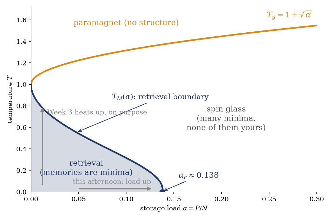
The equations Equation 4.5 are the zero-temperature edge of something larger. Heat the network — we will see in Week 3 that the natural stochastic dynamics at temperature \(T\) exists and is well defined — and the same self-consistent analysis runs at every \((\alpha, T)\). The result is Figure 4.4: a genuine phase diagram for a machine-learning system, computed by Amit, Gutfreund, and Sompolinsky (1985, 1987) with the replica method of spin-glass theory, in the direct lineage of Sherrington and Kirkpatrick (1975). There are three phases. At high temperature, the paramagnet has noise overwhelming any structure, and no memory survives. Below the line \(T_g = 1 + \sqrt{\alpha}\), a spin-glass phase has exponentially many minima, none of them correlated with anything stored — a rugged landscape of pure crosstalk. And in the region under the curve \(T_M(\alpha)\), the retrieval phase has stored patterns as attractors, and the network is a working memory. The retrieval boundary runs from \(T = 1\) at vanishing load down to \(\alpha_c \approx 0.138\) at \(T = 0\) — the capacity \(\alpha_c \approx 0.138\) is the point where the memory phase pinches off against the temperature axis.

The diagram has two natural paths. The horizontal one — loading a cold network with ever more patterns — exits the retrieval phase at \(\alpha_c\); the tutorial follows it. The vertical one — heating a lightly loaded network — shows retrieval surviving to high temperature before melting near \(T \approx 1\); Week 3 follows this path on purpose. The phase diagram also settles a point from the last lecture. Within the retrieval region, a little noise is useful: the spurious attractors — the mixture states of Chapter 3 — are shallower than the retrieval states and melt at lower temperature, so a warm network loses its spurious states while keeping its memories. The same temperature that restores the Boltzmann distribution also cleans the landscape.

Figure 4.4: The phase diagram of the Hopfield model with Hebbian couplings, computed from the finite-temperature replica-symmetric theory of Amit, Gutfreund, and Sompolinsky (1985, 1987) (the boundary \(T_M(\alpha)\) is solved numerically from the self-consistent equations; \(T_g = 1 + \sqrt{\alpha}\)). Below \(T_M(\alpha)\), stored patterns are attractors and the network is a working memory; the retrieval phase ends at \(\alpha_c \approx 0.138\) on the cold axis. Between \(T_M\) and \(T_g\), only spin-glass states survive — many minima, none of them yours. The two gray arrows are the course’s itinerary: the tutorial walks the horizontal path across \(\alpha_c\); Week 3 walks the vertical one, on purpose.

Now we state the debt precisely. What the replica method buys — and what our tools could not — is the average of \(\log Z\) over the stored patterns themselves: the couplings \(J_{ij}\) are random variables built from the \(\xi^\mu\), the free energy must be averaged over that quenched disorder, and for an extensive number of patterns (\(P = \alpha N\)) this average is a nontrivial computation. The technology that computes it — the replica trick, and order parameters beyond \(m\) (the Edwards–Anderson overlap \(q\), and the noise amplification \(r\) you have already met) — is spin-glass theory proper. Module 2 acquires its modern descendants — mean-field theory, its systematic corrections, and the cavity ideas that became inference algorithms — and from that vantage the logic of these equations (feedback, reaction, self-consistency) will be yours to command; the replica computation itself remains, in this course, a named landmark rather than a technique. So Equation 4.5 and Figure 4.4 stand as quoted results, with the physics behind them developed in Module 2’s own language.

One information-theoretic aside, because the number is instructive. At capacity, the network holds \(P \cdot N = 0.138\, N^2\) pattern bits in \(N^2\) real-valued couplings — about \(0.14\) bits per synapse. That is cheap. The optimal capacity of a network permitted to choose its couplings freely — not restricted to Hebb’s one-shot rule — is \(2\) bits per synapse, a bound computed by Elizabeth Gardner in another replica landmark (Gardner 1988) — one this course cites rather than derives. The Hebb rule trades a factor of fifteen in storage efficiency for the privilege of learning in a single pass, with no optimization at all.

Take-home 3

The Hopfield model has a phase diagram: retrieval, spin glass, and paramagnet in the \((\alpha, T)\) plane. Memory is a phase of matter; capacity is its boundary at \(T = 0\). Within the phase, mild noise cleans the landscape — spurious states melt before memories do. The full computation runs on replica machinery (quenched average of \(\log Z\)) that this course quotes rather than builds; Module 2 acquires its modern mean-field descendants.

4.6 Example: the capacity ledger

One concrete network — \(N = 1000\) neurons, the network of Section 3.6 — and every capacity claim of the lecture evaluated on it.

question asked	formula	\(P_\text{max}\)	reading
every pattern letter-perfect	\(N / (4 \ln N)\)	\(\approx 36\)	perfection, all at once
a typical pattern letter-perfect	\(N / (2 \ln N)\)	\(\approx 72\)	perfection, one at a time
retrieval with \(\sim\!2\%\) tolerated error	\(\alpha_c N\), \(\alpha_c \approx 0.138\)	\(\approx 138\)	the AGS answer
Hopfield’s simulation criterion	\(\approx 0.15\, N\) (empirical, \(N=100\))	\(\approx 150\)	finite-size, tolerant
naive iterated map	\((2/\pi)\, N\)	\(\approx 637\)	wrong value, wrong kind

Five numbers for a single network answer three genuinely different questions, with the wrong answer retained as a record of what the naive theory misses. The opening question is settled: Hopfield’s \(0.15\) was the right physics, seen at \(N = 100\) through finite-size rounding, for the tolerant question; sharpened, it is \(0.138\). The strict question was never the one his simulations asked, and its answer is smaller by a logarithm.

The second table makes the same point numerically. For each load: the first-sweep expectation — how many of the \(1000\) bits flip on the first sweep, starting at a stored pattern, from Equation 4.2 — against the true fate of the memory, from Figure 4.3:

\(\alpha = P/N\)	\(P\)	\(P_\text{err}\)	first-sweep flips (of 1000)	true fate
\(0.05\)	\(50\)	\(4 \times 10^{-6}\)	\(\sim 0\)	retrieval, \(m \approx 1\)
\(0.10\)	\(100\)	\(8 \times 10^{-4}\)	\(\sim 1\)	retrieval, \(m\) high
\(0.138\)	\(138\)	\(3.6 \times 10^{-3}\)	\(\sim 4\)	the edge: \(m \approx 0.97\)
\(0.15\)	\(150\)	\(4.9 \times 10^{-3}\)	\(\sim 5\)	dead: \(m \approx 0\)
\(0.20\)	\(200\)	\(1.3 \times 10^{-2}\)	\(\sim 13\)	dead

The \(\alpha = 0.15\) row makes the point. The first sweep gets \(99.5\%\) of the bits right — and the memory is already gone. Between \(138\) and \(150\) patterns, nothing in the per-bit error rate changes appreciably; what changes is that the self-consistent retrieval state stops existing, and the almost-correct first sweep is the first step of an avalanche instead of the last step of a repair. The erfc column is smooth through the transition because the transition was never in it: it lives in the feedback.

Capacity is a phase boundary, not a budget: past it, memory collapses.

The tutorial loads a network at \(N \sim 10^3\) through this exact table; every number required for predicting the results is already in the tables above. The hard problem builds on the warm-up stuck-point card. The week is computation-led, which means the prediction is committed on paper first and each group then runs the sweep itself — one laptop between three or four people, so bring one if you have one.

4.7 Outlook: the partition function returns

Week 2 closes with a substantial inventory. We built a machine out of an Ising model, proved it computes (the Lyapunov theorem), taught it memories in one shot (Hebb), computed what interference costs (today), and found that the machine has a phase diagram in which memory is a phase and forgetting is a phase transition. All of it at zero temperature, with the partition function absent — a stretch of the course where the energy landscape was used bare, with no probability on top.

The step to Week 3 is a single modification. Replace the deterministic update of Equation 3.1 by a stochastic one — flip spin \(k\) with probability

\[ p(s_k \to -s_k) \;=\; \frac{1}{1 + e^{\beta\, \Delta E}}, \]

Glauber dynamics (Week 3)

which needs exactly the \(\Delta E = 2 s_k h_k\) we computed in the Lyapunov derivation, and which reduces to today’s greedy rule as \(\beta \to \infty\). Two statements, both proved in the previous lecture. First, this dynamics has a stationary distribution, and it is \(p(s) \propto e^{-\beta E(s)}\): Week 1’s Boltzmann law returns, now over an energy we designed — the two parts of the course connect. Second, the moment we ask the network to learn its couplings from data by maximum likelihood — rather than have Hebb write them by fiat — the gradient comes out as \(\langle s_i s_j \rangle_\text{data} - \langle s_i s_j \rangle_\text{model}\), and the second average requires sampling from a distribution normalized by \(Z\). That machine is the Boltzmann machine, that gradient is the most transparent learning rule in this course, and that \(Z\) is the obstruction of Week 1, now blocking the training of every energy-based model. Week 3 is where these threads converge.