6The restricted Boltzmann machine: one wall falls, one we walk around
Recommended reading
Core (~1 h).Hinton (2002) — the contrastive-divergence paper and the products-of-experts framing (an RBM is a product of experts, one per hidden unit). This was the warm-up reading, so it is already behind you; re-skim the CD section, which this lecture makes precise. Alongside it, Mehta et al. (2019), §VII — the physicist’s account of the RBM, the factorized conditionals, and CD, in the course’s notation; our derivation follows its logic.
Optional background.Smolensky (1986) — the original “harmonium,” the RBM before it had the name, worth reading for the bipartite idea in its birthplace; Hinton (2012) — the engineering companion, CD-\(k\) in practice and the gap between clean theory and what actually trains; Hinton and Salakhutdinov (2006) — the stacked-RBM result in Science that reignited deep learning, the historical culmination of today’s machinery; MacKay (2003), Ch. 43, for the maximum-likelihood gradient done carefully.
Prerequisite reminder. All of Chapter 5 — the model, the two-phase gradient Equation 5.4, hidden units and the two-expectation problem, and the \(2^N\) ledger — plus the logistic-conditional fact from Section 5.3 and the free energy \(F = -T\log Z\) from Week 1. New today: conditional independence from graph structure, block Gibbs sampling, a closed-form marginal free energy, and the CD-\(k\) approximation with a quantitative account of its bias.
6.1 Two walls, one already read
The previous lecture left the room facing two walls, and we restate them in three lines because today is organized around which of them falls. ① The learning rule: \(\Delta \theta \propto \langle \cdot \rangle_\text{data} - \langle \cdot \rangle_\text{model}\), transparent and exact. ② With hidden units, the positive phase is no longer a lookup: it clamps the visibles and averages over \(p(h \mid v)\) — intractable for a general graph. ③ The negative phase is \(\nabla_\theta \log Z\), a sum over \(2^N\) configurations — intractable regardless of architecture. One wall falls to a theorem and the other we walk around — the difference between exact and approximate.
You have, unusually, already read today’s reading. The warm-up card had you compute \(Z\) for a toy machine with hidden units and watch the sum blow up in your hands, with Hinton (2002) alongside — so you have met both the wall and the workaround’s name. (The natural stuck point is why a short chain is allowed at all — a question the tutorial is built on.) The two results follow: the architecture that makes half the problem exact, and the approximation that makes the other half cheap.
The history has three stages. Smolensky (1986) built the bipartite machine first, inside the connectionist collection that named the era, and called it the harmonium — the restricted Boltzmann machine before it had the name. Hinton (2002) gave it a fast training rule, contrastive divergence, as a by-product of a more general framework (products of experts: the RBM’s hidden units multiply together like independent critics, one constraint each). And in 2006 the combination broke through: Hinton and Salakhutdinov (2006) stacked RBMs, trained them greedily layer by layer with CD, and used the stack to initialize a deep autoencoder that beat PCA soundly — on the pages of Science. That result, with its companion deep-belief-net paper (Hinton, Osindero, and Teh 2006), is widely credited with reigniting deep learning, and the architecture we derive today is where it started.
The thesis: forbidding within-layer connections makes inference exact and sampling fast; computing \(Z\) stays impossible; so we approximate the one average we cannot take — and accept a known bias for a workable algorithm. We are still in Module 1, still at the learned-energy hinge — but this is the module’s first escape technology, and the nature of the escape matters.
Take-home 1
An RBM is a Boltzmann machine with the within-layer couplings removed. That single restriction makes \(p(h \mid v)\) factorize — exact positive phase, fast layer-parallel sampling — while leaving \(Z\) exactly as intractable as in the previous lecture. Architecture defeats one wall exactly; the other admits only approximation.
6.2 Restrict versus approximate
The two moves are independent ideas with opposite characters, and keeping their characters apart is most of the understanding.
The first move is architectural, and exact. Remove the visible–visible and hidden–hidden couplings, and — as we prove in a moment — given one layer, the units of the other become conditionally independent: the clamped positive phase collapses to a formula, and a whole layer can be resampled in one parallel shot. This costs nothing but expressivity-per-layer (recovered, historically, by stacking), and it is a theorem about factorization, not an approximation.
The second move is algorithmic, and biased. No architecture computes \(Z\) — the negative phase still demands equilibrium samples from the model. Contrastive divergence declines to pay for equilibrium: it runs the sampler a few steps from the data and uses whatever it reaches. That is a workaround, and its bias is real; we will quantify it below. Note the independence of the two ideas: CD would apply to any Boltzmann machine; the bipartite structure is what makes CD’s Gibbs steps cheap and the positive phase free. The RBM + CD combination is a fit, not a package deal.
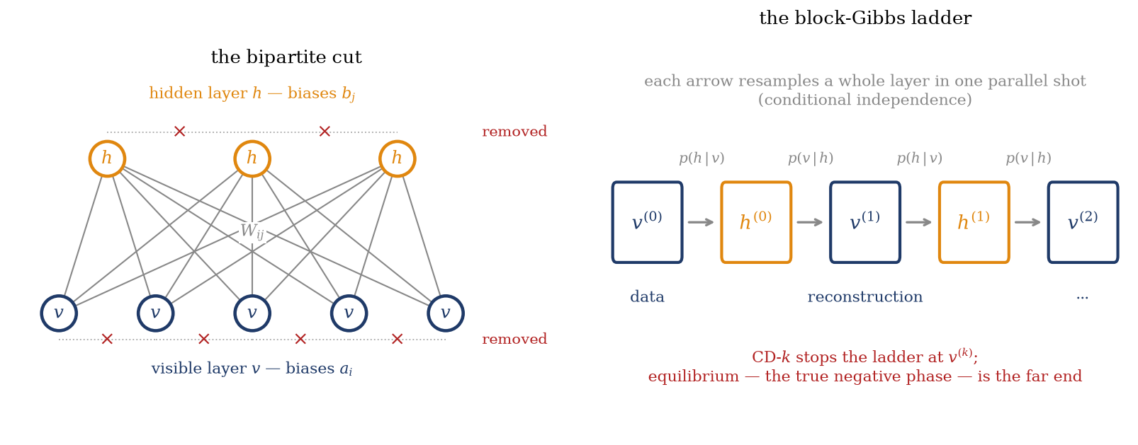
Figure 6.1 draws the central picture — both halves of it. On the left, the bipartite graph: a visible layer \(v\) carrying the data, a hidden layer \(h\), couplings \(W_{ij}\) only between the layers, and the forbidden within-layer edges crossed out — those crosses are the entire design. On the right, the consequence: the block-Gibbs ladder\(v^{(0)} \to h^{(0)} \to v^{(1)} \to h^{(1)} \to \cdots\), each arrow resampling one full layer from its factorized conditional. The next section treats the left half (why the layers factorize, and what that buys), and contrastive divergence is a statement about the right half (how far up the ladder we bother to climb).
Figure 6.1: The central picture of the lecture. Left: the bipartite cut — visible units \(v\) (biases \(a_i\)), hidden units \(h\) (biases \(b_j\)), weights \(W_{ij}\) only between the layers; the crossed-out within-layer edges are the restriction that gives the RBM its name and all of its tractability. Right: the block-Gibbs ladder — because each layer is conditionally independent given the other, the alternating chain \(v^{(0)} \to h^{(0)} \to v^{(1)} \to \cdots\) resamples a whole layer per arrow. The data sit at \(v^{(0)}\); the one-step reconstruction is \(v^{(1)}\); the true negative phase lives at the far, equilibrium end of the ladder — and CD-\(k\) stops climbing after \(k\) rungs.
6.3 The engine: bipartite structure and its consequences
The previous lecture’s obstacle: the hidden-unit positive phase needed \(p(h \mid v)\), intractable on a general graph. What is the least structure we can remove to make that conditional trivial? Answer: the within-layer edges — and here is why.
Setup, with a convention shift flagged. RBM units are binary \(\{0, 1\}\) — active or silent — rather than the \(\pm 1\) spins of Weeks 2–3. This is the convention of the entire RBM literature and of the tutorial, so we adopt it; the affine map \(s = 2v - 1\) converts one convention to the other, renormalizing couplings and shuffling constants into the biases (mix the two silently and it is precisely the biases that get corrupted). With visible biases \(a_i\), hidden biases \(b_j\), and a weight matrix \(W_{ij}\), the energy is
— no \(v_i v_{i'}\) terms, no \(h_j h_{j'}\) terms. The key observation is immediate: for fixed \(v\), this energy is linear in \(h\) (and symmetrically, for fixed \(h\), linear in \(v\)). Group the \(h\)-dependent terms accordingly,
\(c_j(v)\): the effective field on hidden unit \(j\)
where \(c_j(v)\) collects everything hidden unit \(j\) feels — its bias plus the weighted activity of the visible layer.
The conditional factorizes. Compute \(p(h \mid v)\) head-on. The factor \(e^{\sum_i a_i v_i}\) is common to numerator and denominator and cancels; what remains splits per hidden unit, because both the exponential of a sum and the sum over \(h \in \{0,1\}^{n_h}\) factorize:
In words: given the other layer, each unit is an independent logistic neuron — the sigmoid of Section 5.3, a conditional Boltzmann probability for one two-state degree of freedom in the field of its neighbors, now sitting inside a learning machine. Conditional independence is the consequence of the bipartite cut, and it has three uses.
The positive phase is exact. Clamp \(v\) to a data point. Because the \(h_j\) are independent given \(v\), the clamped expectation needs no sum over hidden configurations at all: \(\langle v_i h_j \rangle_{h \mid v} = v_i\, \sigma(c_j(v))\), a number. Averaging over the training set,
— no sampling, no \(Z\), cost linear in the dataset. The wall the previous lecture raised for the general graph is gone, by structure. (This is also, note, the general two-phase gradient of Section 5.6 specialized to the RBM: \(\partial \log p(v)/\partial W_{ij} = \langle v_i h_j \rangle_\text{data} - \langle v_i h_j \rangle_\text{model}\), with the first bracket now a formula.)
Block Gibbs sampling. The same independence makes the sampler fast: draw all of \(h\) from \(p(h \mid v)\) in one parallel shot (\(n_h\) independent coin flips with probabilities \(\sigma(c_j)\)), then all of \(v\) from \(p(v \mid h)\), and alternate — the ladder of Figure 6.1. Each half-update resamples a block of variables from its exact conditional, which leaves the joint \(p(v, h) = e^{-E}/Z\) invariant (resampling \(h\) from \(p(h \mid v)\) cannot change a distribution that already factorizes as \(p(v)\,p(h \mid v)\) — the one-line stationarity argument; irreducibility and aperiodicity hold as in Section 5.3 since every conditional probability is strictly positive). This is Glauber’s dynamics (Glauber 1963) upgraded from one spin per move to one layer per move — the sampler that every downstream method, starting with CD, will lean on.
Tracing out the hidden layer. The factorized sum that gave us the conditionals gives us one more thing, and it is a result of directly statistical-mechanical character. Sum the joint weight over all hidden configurations — the same per-unit split as before:
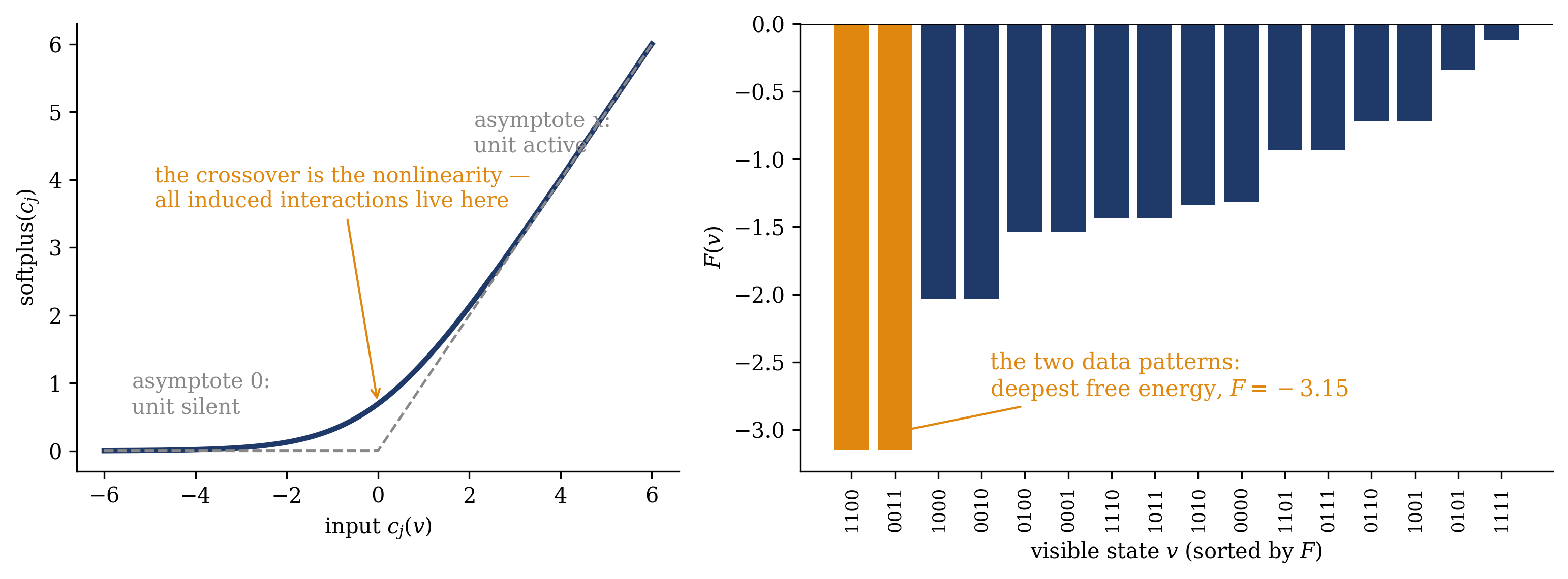
Physically, \(F(v) = -\log \sum_h e^{-E(v,h)}\) is a free energy — we integrated out the hidden (“fast”) degrees of freedom to obtain an effective theory over the visible (“slow”) ones, the same coarse-graining move statistical mechanics makes whenever it trades microscopic detail for an effective potential. Each hidden unit contributes one softplus term — Figure 6.2 draws the function and the landscape it builds — and the softplus is where the previous lecture’s promise is kept: \(c_j(v)\) is linear in \(v\), but \(\operatorname{softplus}\) is not, and expanding it generates products of visibles of all orders. The effective higher-order interactions that hidden units were bought for are now explicit, computable, and sitting in one line.
The contrast is immediate. \(F(v)\) is a closed-form expression — evaluate it at any \(v\) in microseconds. The normalizer \(Z = \sum_v e^{-F(v)}\) is a sum over \(2^{n_v}\) visible configurations — as intractable as ever. Everything about this model is computable except its normalizer.
Show code
fig, (a1, a2) = plt.subplots(1, 2, figsize=(10.4, 3.9), width_ratios=[1, 1.25])xx = np.linspace(-6, 6, 400)a1.plot(xx, np.log1p(np.exp(xx)), color=NAVY, lw=2.5)a1.plot(xx, np.where(xx >0, xx, 0), color=GRAY, ls="--", lw=1.2)a1.text(-5.4, 0.55, "asymptote $0$:\nunit silent", color=GRAY, fontsize=10)a1.text(2.1, 4.4, "asymptote $x$:\nunit active", color=GRAY, fontsize=10)a1.annotate("the crossover is the nonlinearity —\nall induced interactions live here", xy=(0, 0.69), xytext=(-4.9, 3.6), color=ORANGE, fontsize=10, arrowprops=dict(arrowstyle="->", color=ORANGE, lw=1))a1.set_xlabel(r"input $c_j(v)$"); a1.set_ylabel(r"$\operatorname{softplus}(c_j)$")order = np.argsort(F)lbl = ["".join(str(int(x)) for x in V[c]) for c in order]colors = [ORANGE if l in ("1100", "0011") else NAVY for l in lbl]a2.bar(range(16), F[order], color=colors)a2.set_xticks(range(16), lbl, rotation=90, fontsize=8.5)a2.axhline(0, color="k", lw=0.8)a2.annotate("the two data patterns:\ndeepest free energy, $F=-3.15$", xy=(0.5, -3.05), xytext=(3.2, -2.75), color=ORANGE, fontsize=10.5, arrowprops=dict(arrowstyle="->", color=ORANGE, lw=1))a2.set_xlabel(r"visible state $v$ (sorted by $F$)"); a2.set_ylabel(r"$F(v)$")fig.tight_layout(); plt.show()
Figure 6.2: The coarse-graining, drawn. Left: \(\operatorname{softplus}(x) = \log(1+e^x)\), the effective potential a single hidden unit contributes to \(F(v)\) once traced out — flat (\(\approx 0\)) when its input is strongly negative, linear (\(\approx x\)) when strongly positive, with the crossover at \(c_j = 0\) carrying all the nonlinearity (and hence all the induced higher-order interactions among the visibles). Right: the free energy Equation 6.4 of the small RBM of Section 6.6, evaluated in closed form at all \(2^4 = 16\) visible states: the two data patterns \((1100)\) and \((0011)\) are the two deepest states at \(F = -3.15\). Every bar is a microsecond’s arithmetic; the sum \(Z = \sum_v e^{-F(v)}\) over the bars is what remains intractable at scale.
Trap
Conditional independence is not marginal independence.\(p(h \mid v)\) factorizes; \(p(v)\), \(p(v, h)\), and above all \(Z\) do not — the visibles are strongly coupled through the hidden units they share (that coupling is the model’s entire expressive power), and \(Z\) is still a sum over exponentially many states. “The RBM’s partition function factorizes” is the most tempting wrong sentence of the week. The conditionals factorize; the partition function does not.
6.4 Contrastive divergence: dodging the negative phase
Here the lecture changes character: we stop deriving exact results and start approximating. The RBM’s structure fixed the positive phase; the negative phase \(\langle v_i h_j \rangle_\text{model}\) is untouched — it wants an average over the free-running model, which means block Gibbs run to equilibrium, at every gradient step, on a landscape that (Week 2) may mix exponentially slowly. Equilibrium is the cost we now refuse to pay. The question Hinton (2002) asked: what if we run the ladder just a little?
The CD-\(k\) rule. Start the Gibbs chain at a data point — not at a random state — and climb \(k\) rungs of the ladder: \(v^{(0)} = v_\text{data} \to h^{(0)} \to v^{(1)} \to \cdots \to v^{(k)}\). Then estimate the negative phase from where the chain got to:
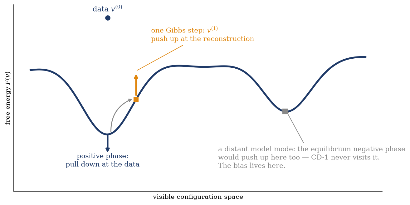
with both brackets evaluated by the exact formula Equation 6.3 (using the hidden probabilities\(\sigma(c_j)\) rather than sampled \(h_j\) cuts variance at no cost in expectation — standard practice (Hinton 2012)). CD-1 — one up–down–up pass — is the workhorse: the negative sample is the model’s one-step reconstruction of the data, and the update pushes energy down at the data and up at the reconstruction. Figure 6.3 places the move on the free-energy landscape, and against the previous lecture’s global picture.
Figure 6.3: What CD-1 actually does, drawn on the visible free-energy landscape \(F(v)\) — compare Figure 5.2, where the negative phase pushed up at all the model’s modes. CD starts at the data, takes one Gibbs step, and pushes up at the resulting reconstruction: a local negative phase, applied where the model’s probability mass sits near the data. If the model is right, the step doesn’t move (\(v^{(1)} \approx v^{(0)}\)) and the two arrows cancel. The price is drawn in gray: a distant spurious mode that equilibrium sampling would find and suppress is never visited by a short chain — CD’’s bias lives exactly there.
Why starting at the data is the clever part. There are two readings, one cheap and one deep. The cheap one: a chain started at the data begins in a high-probability region of a decent model, so \(k\) steps of honest Gibbs produce a sample that is “trying” to equilibrate locally — far better than \(k\) steps from a random state, which would still be essentially noise. The deep one: if the model were perfect, the data would already be an equilibrium sample, one Gibbs step would leave its distribution unchanged, the two brackets in Equation 6.5 would agree in expectation, and the update would vanish. The maximum-likelihood solution is therefore (approximately) a fixed point of CD — the rule is engineered to stop pushing exactly when there is nothing left to learn. When the model is wrong, one step drifts the data toward the model’s nearby fantasies, and CD raises the energy precisely there: a negative phase sampled where it matters most, at the front line between data and model, rather than uniformly over the model’s whole support.
The price, stated precisely. CD is biased, and the bias is not a rounding error — it is structural, and three progressively sharper statements pin it down. First, the CD-\(k\) update is not the gradient of the log-likelihood: the true negative phase averages over the model everywhere; CD’s averages only over what a \(k\)-step chain reaches (the gray mode of Figure 6.3 is real, and a landscape’s distant spurious modes are exactly what short chains never police). Hinton’s own motivation — that CD-\(k\) approximately descends the contrastive objective \(D_\mathrm{KL}(p_0 \| p_\infty) - D_\mathrm{KL}(p_k \| p_\infty)\), the amount by which \(k\) Gibbs steps move the data distribution toward the model — is illuminating but heuristic, and he said so (Hinton 2002). Second, it is not the gradient of that objective either, nor of any objective: Sutskever and Tieleman (2010) showed the CD update is not the gradient of any function at all — there is no hidden loss being optimized. Third, the effect is measurable: the fixed points of CD learning differ from the maximum-likelihood solutions, an effect analyzed and quantified on exactly-solvable small models by Carreira-Perpiñán and Hinton (2005) — whose diagnosis is also the reassurance: the bias is usually small, shrinks as \(k\) grows (as \(k \to \infty\) the chain equilibrates and CD-\(k\)is maximum likelihood), and rarely matters for learning good features, though it does distort the learned distribution.
The standard modern mitigation costs one sentence: persistent CD(Tieleman 2008) keeps a set of “fantasy” chains running across parameter updates — never resetting to the data — so the negative-phase samples track the slowly moving model far better than a freshly truncated chain, at essentially no extra cost. (The chains stay approximately equilibrated because each parameter update moves the model only slightly — an adiabatic argument a physicist will recognize.)
Trap
CD never computes \(Z\) — and never estimates it. It sidesteps the negative-phase expectation by sampling; the normalizer itself is untouched, unknown, and unknowable at scale. Corollary: you cannot evaluate the likelihood of a trained RBM either — training monitors proxies (reconstruction error, pseudo-likelihood), and a low reconstruction error is not a high likelihood: a model can reconstruct data beautifully while assigning most of its probability mass to garbage it never shows you. Mistaking the proxy for the objective is the standard failure mode of energy-based practice. (How one does estimate \(Z\) when it truly matters — annealed importance sampling — is Week 11’s fluctuation-theorem machinery; noted, not developed.)
Take-home 2
Contrastive divergence estimates the negative phase from a short Gibbs chain started at the data: \(\Delta W_{ij} \propto \langle v_i h_j \rangle_\text{data} - \langle v_i h_j \rangle_{v^{(k)}}\). It trades an unbiased-but-intractable gradient for a biased-but-cheap one; the bias is real (CD is not maximum likelihood — not even the gradient of any objective — and its fixed points differ), shrinks with \(k\), and is mitigated by persistent chains. CD dodges\(Z\); it never computes it.
6.5 From workaround to revival
What the workaround bought warrants two paragraphs of history, because they explain why a superseded model still owns a week of the course.
Through the 1990s and early 2000s, deep networks could not be trained: backpropagation through many layers lost its gradient, and every serious attempt stalled. The RBM + CD combination broke the deadlock from an unexpected side. Hinton and Salakhutdinov (2006) trained a stack of RBMs greedily — each layer learned, by CD, to model the hidden activities of the layer below — then unrolled the stack into a deep autoencoder and fine-tuned; the pretrained network compressed images and documents better than PCA, and, decisively, trained at all. The companion paper (Hinton, Osindero, and Teh 2006) built generative deep belief nets the same way. For roughly five years, greedy layer-wise RBM pretraining was how one trained anything deep — until better activations, initializations, optimizers, and GPUs (circa 2012) made the scaffolding unnecessary, and the field moved on.
The current status, then: as production models, RBMs and CD are historical — you will not deploy one, and this course will not pretend otherwise. We spend a week on them because they are the cleanest habitat of ideas the course cannot do without: energy-based learning, the two-phase gradient, the \(Z\) obstruction, sampling as the price of normalization, and contrastive estimation — the move of pitting data against the model’s own samples, which echoes through noise-contrastive estimation, GAN discriminators, and the negative sampling of modern representation learning. The RBM is to energy-based learning what the Ising model is to phase transitions: nobody’s production system, everybody’s understanding.
Normative practice, for the record and the tutorial (the flat ranking a practitioner actually uses): for feature learning, CD-1 is usually enough — its bias barely touches the filters. For generation, use CD-\(k\) with \(k\) in the tens, or better, persistent CD. Sample the hidden states when they are driven by the data — the stochastic binary bottleneck is what stops each hidden unit from passing more than a bit, and all-probabilities chains collapse into deterministic mean-field fixed points — but use probabilities, not samples, for the visible reconstructions and for the hidden activities that enter the final gradient statistics. Monitor reconstruction error and pseudo-likelihood knowing they are proxies, and watch for the signature failure where reconstruction keeps improving while the model’s samples degrade. All of it is systematized in Hinton (2012) — the rare paper that is accurately titled a practical guide. (Script asides, named for completeness: real-valued data uses Gaussian-visible RBMs — binary units are a choice, not a law; and the closed-form \(F(v)\) makes a trained RBM usable as a classifier by comparing free energies of label-conditioned configurations.)
6.6 Example: watching the bias
One concrete RBM, small enough to enumerate, so that the CD bias — invisible in any real application, because seeing it requires the very sum CD exists to avoid — is visible. Take \(n_v = 4\) visible and \(n_h = 3\) hidden units: \(2^{4+3} = 128\) joint states, comfortably inside the enumerable region of the previous lecture’s ledger (Section 5.7). The machine is hand-built to be legible: hidden unit 1 is tuned to the pattern “left pair on” (\(W_{\cdot 1} = (2, 2, -2, -2)\)), hidden unit 2 to “right pair on” (\(W_{\cdot 2} = (-2, -2, 2, 2)\)), hidden unit 3 weakly coupled (\(W_{\cdot 3} = (0.5, -0.5, 0.5, -0.5)\)); biases \(a_i = -0.3\), \(b = (-1, -1, 0)\). The dataset is six points in two clusters — four copies of \((1,1,0,0)\), two of \((0,0,1,1)\). This is a machine already well adapted to its data: brute force gives \(Z = 98.9\), and the two data patterns are the two lowest-free-energy states of Figure 6.2, each carrying \(p(v) = 0.236\) of the model’s mass — though note the model splits its mass symmetrically while the data arrive 4 : 2, so there is still something to learn, and the exact gradient will point at it.
For the single weight \(W_{11}\) (first visible unit, first hidden unit), the three ways of producing the two brackets of Equation 6.5:
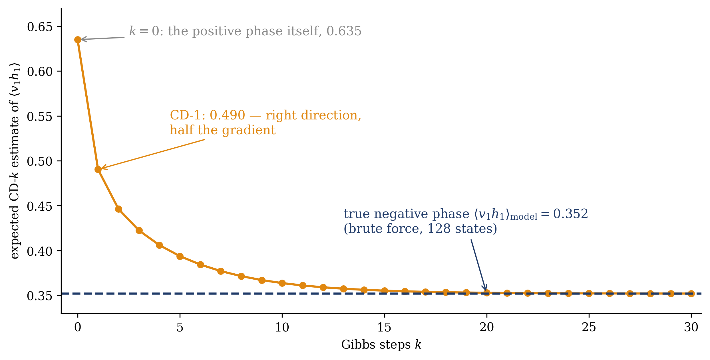
(For the CD row we tabulate the expected CD-1 estimate — the data distribution propagated exactly through one block-Gibbs step, so the number is deterministic; a sampled run scatters around it.) Read the columns across. The positive phase is the truth — exact by Equation 6.3, at trivial cost; e.g. clamping \(v = (1,1,0,0)\) gives \(\sigma(c_1) = \sigma(3) = 0.95\), hidden unit 1 all but certainly on. The middle column is the truth CD cannot afford: at \(128\) states we can buy it; at \(128\) units we never will. And the CD-1 column approximates the middle column while leaning toward the first: one Gibbs step has not carried the data far into the model, and the reconstruction statistics still remember where they started. The resulting gradients: exact, \(0.635 - 0.352 = +0.283\); CD-1, \(0.635 - 0.490 = +0.145\). The CD-1 gradient has the right sign at half the size: it learns in the correct direction and undershoots, which is very much its general character.
As the chain climbs the ladder, the bias drains: Figure 6.4 plots the expected CD-\(k\) estimate against \(k\), sliding from the data value at \(k = 0\) (the estimate before any Gibbs step is the positive phase) to the exact negative phase as \(k \to \infty\):
\(k\)
expected CD-\(k\) estimate
bias
\(1\)
\(0.490\)
\(+0.138\)
\(2\)
\(0.446\)
\(+0.094\)
\(5\)
\(0.394\)
\(+0.042\)
\(10\)
\(0.364\)
\(+0.012\)
\(20\)
\(0.353\)
\(+0.001\)
The decay is controlled by the chain’s mixing: this machine’s couplings (\(|W| = 2\)) carve two well-separated modes, and a chain started in one takes many rungs to visit the other in fair proportion — the previous lecture’s second obstruction, sampling hardness, quietly setting the price of CD’s shortcut. Strengthen the couplings and the bias at fixed \(k\) grows; this is the toy version of why CD struggles precisely on the strongly structured models one most wants.
Show code
# exact block-Gibbs transition matrix on the visibles: T[v, v'] = sum_h p(h|v) p(v'|h)ph_v = np.prod(sig(C)[:, None, :] ** H[None, :, :]* (1- sig(C))[:, None, :] ** (1- H[None, :, :]), axis=2) # 16 x 8Ah = H @ W.T + apv_h = np.prod(sig(Ah)[:, None, :] ** V[None, :, :]* (1- sig(Ah))[:, None, :] ** (1- V[None, :, :]), axis=2) # 8 x 16T = ph_v @ pv_hE = np.array([[-(v @ a) - (h @ b) - v @ W @ h for h in H] for v in V])p_joint = np.exp(-E) / np.exp(-E).sum()neg_exact = np.einsum("vh,vi,hj->ij", p_joint, V, H)[0, 0] # 0.352p0 = np.zeros(2**nv) # empirical data distributionfor d in data: p0[int(sum(int(x) << i for i, x inenumerate(d)))] +=1/len(data)ks = np.arange(0, 31)est, pk = [], p0.copy()for k in ks: est.append(np.einsum("v,v,v->", pk, V[:, 0], sig(C)[:, 0])) pk = pk @ Test = np.array(est)fig, ax = plt.subplots(figsize=(8.4, 4.3))ax.plot(ks, est, "o-", color=ORANGE, lw=1.8, ms=5)ax.axhline(neg_exact, color=NAVY, ls="--", lw=1.8)ax.annotate(rf"true negative phase $\langle v_1 h_1\rangle_\mathrm{{model}} = {neg_exact:.3f}$""\n(brute force, 128 states)", xy=(20, neg_exact), xytext=(13, 0.42), color=NAVY, fontsize=10.5, arrowprops=dict(arrowstyle="->", color=NAVY, lw=1))ax.annotate(r"$k=0$: the positive phase itself, $0.635$", xy=(0, est[0]), xytext=(2.5, 0.64), color=GRAY, fontsize=10.5, arrowprops=dict(arrowstyle="->", color=GRAY, lw=1))ax.annotate(rf"CD-1: ${est[1]:.3f}$ — right direction,""\nhalf the gradient", xy=(1, est[1]), xytext=(4.5, 0.53), color=ORANGE, fontsize=10.5, arrowprops=dict(arrowstyle="->", color=ORANGE, lw=1))ax.set_xlabel(r"Gibbs steps $k$")ax.set_ylabel(r"expected CD-$k$ estimate of $\langle v_1 h_1\rangle$")ax.set_xlim(-0.8, 30.5); ax.set_ylim(0.33, 0.67)fig.tight_layout(); plt.show()
Figure 6.4: The CD-\(k\) bias, exactly, on the enumerable RBM of this section (\(n_v = 4\), \(n_h = 3\); \(Z = 98.9\)). Orange: the expected CD-\(k\) estimate of the negative phase \(\langle v_1 h_1 \rangle\), computed by propagating the data distribution through \(k\) exact block-Gibbs steps (no sampling noise). At \(k = 0\) the estimate is the positive phase itself (\(0.635\)); as \(k \to \infty\) the chain equilibrates onto the true negative phase (\(0.352\), navy dashed). CD-1 stops one rung up the ladder at \(0.490\) — right direction, roughly half the true gradient — and the bias decays with \(k\) at a rate set by how fast the chain mixes between the machine’s two modes. On this toy we can see the whole curve; on any real model, only the \(k\) we pay for.
The tutorial (16–18, Ph12 106) runs on exactly this machinery, scaled up: a real RBM, CD-1 against CD-10, learned filters and sampled fantasies side by side. Your job in the room is to predict which is which, and why, before anything renders — the prediction is committed on paper, and only then does each group open a machine and run it. Every formula required is already in this chapter. The hard problem builds on the warm-up’s stuck point.
The conditionals factorize; the partition function does not — that gap is exactly what we approximate.
Take-home 3
On a brute-forceable RBM the three columns are all visible: the positive phase is exact by formula, the negative phase is exact by enumeration, and CD-1 approximates the latter with a bias that leans toward the data — right sign, wrong magnitude, decaying with \(k\) at the chain’s mixing rate. The bias is the measurable price of dodging \(Z\) — visible here because the model is tiny, invisible and unavoidable when it is not.
6.7 Outlook: where the obstruction stands
The previous lecture derived the learning rule and the obstruction. Today the positive-phase wall fell — to a theorem, the bipartite factorization, at no cost in exactness — and the negative-phase wall was walked around — by contrastive divergence, at the cost of a real, quantified bias. The partition function itself is exactly as intractable as it was in the previous lecture: we have become good at avoiding\(Z\), not at computing it. That asymmetry reflects the state of the field, and every module until Week 10 is a better avoidance — mean-field and variational bounds in Module 2, smarter sampling in Module 3.
Next week the energy-based view scales to the present: modern Hopfield networks carry an energy whose capacity is exponential rather than \(0.138\,N\), and whose retrieval update turns out to be exactly the attention mechanism of the transformer. Week 2’s machine never went away; Week 4 makes the connection precise. And Week 10 keeps the promise the previous lecture made precise: score matching trades \(\nabla_\theta \log Z\), which is intractable, for \(\nabla_x \log Z\), which is zero — not another approximation but a resolution (Hyvärinen 2005). CD postpones the negative phase; score matching dissolves it.
Carreira-Perpiñán, Miguel Á., and Geoffrey E. Hinton. 2005. “On Contrastive Divergence Learning.” In Proceedings of the 10th International Workshop on Artificial Intelligence and Statistics (AISTATS), R5:33–40. Proceedings of Machine Learning Research.
Glauber, Roy J. 1963. “Time-Dependent Statistics of the Ising Model.”Journal of Mathematical Physics 4 (2): 294–307. https://doi.org/10.1063/1.1703954.
Hinton, Geoffrey E. 2002. “Training Products of Experts by Minimizing Contrastive Divergence.”Neural Computation 14 (8): 1771–1800. https://doi.org/10.1162/089976602760128018.
———. 2012. “A Practical Guide to Training Restricted Boltzmann Machines.” In Neural Networks: Tricks of the Trade, edited by Grégoire Montavon, Genevieve B. Orr, and Klaus-Robert Müller, 2nd ed., 7700:599–619. Lecture Notes in Computer Science. Springer. https://doi.org/10.1007/978-3-642-35289-8_32.
Hinton, Geoffrey E., Simon Osindero, and Yee-Whye Teh. 2006. “A Fast Learning Algorithm for Deep Belief Nets.”Neural Computation 18 (7): 1527–54. https://doi.org/10.1162/neco.2006.18.7.1527.
Hinton, Geoffrey E., and Ruslan R. Salakhutdinov. 2006. “Reducing the Dimensionality of Data with Neural Networks.”Science 313 (5786): 504–7. https://doi.org/10.1126/science.1127647.
Hyvärinen, Aapo. 2005. “Estimation of Non-Normalized Statistical Models by Score Matching.”Journal of Machine Learning Research 6: 695–709.
MacKay, David J. C. 2003. Information Theory, Inference, and Learning Algorithms. Cambridge: Cambridge University Press.
Mehta, Pankaj, Marin Bukov, Ching-Hao Wang, Alexandre G. R. Day, Clint Richardson, Charles K. Fisher, and David J. Schwab. 2019. “A High-Bias, Low-Variance Introduction to Machine Learning for Physicists.”Physics Reports 810: 1–124. https://doi.org/10.1016/j.physrep.2019.03.001.
Smolensky, Paul. 1986. “Information Processing in Dynamical Systems: Foundations of Harmony Theory.” In Parallel Distributed Processing: Explorations in the Microstructure of Cognition, Vol. 1, edited by David E. Rumelhart and James L. McClelland, 194–281. Cambridge, MA: MIT Press.
Sutskever, Ilya, and Tijmen Tieleman. 2010. “On the Convergence Properties of Contrastive Divergence.” In Proceedings of the 13th International Conference on Artificial Intelligence and Statistics (AISTATS), 9:789–95. Proceedings of Machine Learning Research.
Tieleman, Tijmen. 2008. “Training Restricted Boltzmann Machines Using Approximations to the Likelihood Gradient.” In Proceedings of the 25th International Conference on Machine Learning (ICML), 1064–71. https://doi.org/10.1145/1390156.1390290.