12 Belief propagation: the cavity becomes an algorithm

12.1 Passing the cavity field

The previous lecture’s cavity field — the field on a spin computed in the cavity where that spin is removed — is, in structure, a message. Today the identification becomes precise, and the consequences run through the rest of the week. Compute the cavity field not once, as a correction, but recursively, along the edges of a graph: every node tells every neighbor what it believes in that neighbor’s absence, each such report built from the reports the node itself received from everyone else. Iterate to consistency. That is belief propagation, and on a tree it is not an approximation at all — it returns the exact marginals of a \(2^N\)-state distribution in a number of operations linear in \(N\). (One question suggests itself immediately: what is a message, if not a marginal? The difference between the two is the entire method.)

The history is the course’s thesis in miniature, because this algorithm was invented three times, in three fields that were not talking to each other. Bethe (1935) invented it in statistical physics, as an approximation for alloys — the “Bethe approximation” whose free energy we meet today. Gallager (1962) invented it in coding theory, as an iterative decoder for the error-correcting codes that were decades ahead of their hardware — the LDPC codes that now run in your phone’s radio. And Pearl (1988) invented it in artificial intelligence, as exact inference on the graphical models that organized modern probabilistic reasoning. Three communities and three notations converged on one algorithm — and the demonstration that they are one thing, assembled in the book you read for the warm-up (Mézard and Montanari 2009), is as sharp a statement of this course’s premise as any: physics, coding, and inference are one subject speaking three languages.

The driving question picks up where the previous lecture’s verdict left off. TAP’s reaction term was the right correction for a dense graph — the Plefka expansion said so. But the graphs of real inference problems are not all dense: they are sparse, structured, tree-like, loopy. What is the right correction for an arbitrary graph? Today’s answer is structural rather than perturbative: Pass the cavity field along each edge and let the graph itself decide — on a tree the result is exact, and on a dense graph, at the end of the lecture, the messages collapse and their correction is the Onsager term. Message passing contains TAP.

Take-home 1

Belief propagation is the previous lecture’s cavity field, passed recursively along a graph’s edges: each node tells each neighbor what it believes in that neighbor’s absence. On a tree it returns the exact marginals — and it was invented three separate times (Bethe 1935, Gallager 1962, Pearl 1988) because physics, coding, and inference are one problem.

12.2 Node beliefs versus edge messages

One structural dichotomy organizes the method and is worth stating before the algebra. Week 5’s mean field tracked one number per node — the magnetization \(m_i\) — and paid for that economy with zero correlations. Belief propagation tracks one number per directed edge: the message \(u_{k\to i}\), a different report for every recipient, because what \(k\) believes in \(i\)’s absence genuinely depends on who \(i\) is. That per-edge bookkeeping is exactly what lets correlation flow along the graph — and it is the previous lecture’s cavity distinction (\(m_j\) versus \(m_j^{(i)}\)), promoted from a second-order correction to the method’s primary variable.

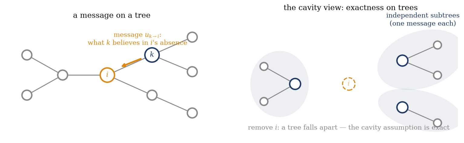
Figure 12.1 draws the central picture, both halves. Left: a tree, with one message flowing along one directed edge — \(u_{k \to i}\), everything the subtree behind \(k\) has to say to \(i\), condensed into a single effective field. Right: the reason trees are special. Remove node \(i\), and a tree falls apart — the neighbors’ subtrees are genuinely, exactly independent of one another, because the only path between them ran through \(i\). The cavity assumption that the previous lecture’s TAP invoked approximately (“the neighbors are independent in my absence”) is, on a tree, simply true. The results of this lecture follow from that picture: exactness where removing a node disconnects, correction terms where it does not.

Figure 12.1: The central picture of the lecture. Left: a message on a tree — \(u_{k\to i}\) carries everything the subtree behind \(k\) has to say to \(i\), condensed into one effective field: *what \(k\) believes in \(i\)’s absence*. Right: why trees are special — remove \(i\) and the tree falls apart into independent subtrees, one per neighbor, each summarized by one incoming message. The cavity assumption (“my neighbors are independent in my absence”) is exactly true on a tree; every loop in a graph is a way for it to fail.

12.3 The engine: belief propagation

Setup. A pairwise model on a graph — Ising, for concreteness and continuity: spins \(s_i = \pm 1\), couplings \(J_{ij}\) on the edges, fields \(h_i\), temperature \(T\) live as it has been all module. Write \(\partial i\) for the set of \(i\)’s neighbors. Two cavity objects, and then the recursion closes on itself.

The cavity field, per edge. Let \(h_{i \to j}\) be the effective field on \(i\) with the edge to \(j\) cut — the previous lecture’s cavity field, now directed. In the cavity, \(i\)’s remaining neighbors act on it independently (exactly so on a tree), so their contributions add.

The message. What does neighbor \(k\) contribute to \(i\)? Trace \(k\) out. Spin \(k\) sits in its own cavity field \(h_{k \to i}\) (its field from everything except \(i\)) and couples to \(i\) through \(J_{ki}\); summing over \(s_k = \pm 1\) produces an effective field on \(i\), and two lines of algebra give it in closed form. Define \(u_{k\to i}\) by \(\sum_{s_k} e^{\beta J_{ki} s_k s_i + \beta h_{k\to i} s_k} \propto e^{\beta u_{k \to i} s_i}\); taking the ratio of the \(s_i = \pm 1\) cases,

\[ e^{2\beta u_{k\to i}} = \frac{\cosh\beta(h_{k\to i} + J_{ki})}{\cosh\beta(h_{k\to i} - J_{ki})} \qquad\Longrightarrow\qquad \tanh(\beta u_{k\to i}) = \tanh(\beta J_{ki})\,\tanh(\beta h_{k\to i}), \]

that is,

\[ \boxed{\; u_{k \to i} \;=\; \frac{1}{\beta}\, \operatorname{artanh}\!\Big[ \tanh(\beta J_{ki})\, \tanh\big(\beta\, h_{k \to i}\big) \Big] \;} \tag{12.1}\]

BP message: what \(k\) tells \(i\)

In words: the message is \(k\)’s cavity magnetization \(\tanh(\beta h_{k\to i})\), attenuated by the bond through \(\tanh(\beta J_{ki})\) — a weak bond transmits almost none of \(k\)’s belief, a strong bond passes it on nearly verbatim, and the \(\operatorname{artanh}\) converts the result back into field units so that messages can be added.

The recursion, and the marginals. The cavity field on \(i\) toward \(j\) collects the messages from all of \(i\)’s other neighbors,

\[ h_{i \to j} \;=\; h_i + \sum_{k \in \partial i \setminus j} u_{k \to i}, \]

and the definition closes on itself: messages determine cavity fields determine messages. Iterate to a fixed point (sweep the directed edges; damping helps on hard instances, as it did in the previous lecture). Once converged, the full marginal at a node combines all incoming messages:

\[ m_i \;=\; \tanh\!\Big( \beta \Big[ h_i + \sum_{k \in \partial i} u_{k \to i} \Big] \Big) \tag{12.2}\]

BP marginal: all messages combined

And here is the promised answer to the opening question. A message is not a marginal. The message \(u_{k\to i}\) is a belief in \(i\)’s absence — computed from \(h_{k \to i}\), which deliberately excludes what \(i\) itself has been telling \(k\). The marginal \(m_i\) is what you believe once every neighbor has told you what they believe without you. Keeping the two straight — always asking “who was removed?” — is precisely the discipline that prevents the double-counting the previous lecture was about. A node that fed its own message back into the reply it receives would be responding to its own echo.

Exactness on trees. Now the theorem, and after Figure 12.1 it is one paragraph. The only assumption anywhere above is the cavity assumption: that \(i\)’s neighbors are statistically independent once \(i\) is removed. On a tree, removing \(i\) disconnects the neighbors’ subtrees — there is no path left between them — so the assumption is exactly true, at every node, at every step of the recursion. By induction from the leaves (whose cavity fields are just their local fields, no assumption needed), every message is exact, hence every marginal Equation 12.2 is exact. A \(2^N\)-sum inference problem, solved in \(\mathcal{O}(N)\) message updates, with no approximation: belief propagation on a tree is an exactly solvable algorithm. And the same paragraph locates the failure mode in advance: on a graph with loops, removing \(i\) does not disconnect its neighbors — influence can travel around the loop and return — which is exactly the self-reaction that trees lack and the previous lecture subtracted. Loops are where messages become echoes.

The oldest special case: the chain. The simplest tree has no branching at all, and on it the theorem lands on an algorithm invented yet a fourth time, in yet a fourth field (Welling, Lu, and Holdijk 2026, ch. 6 on belief propagation). Consider a hidden Markov model, the workhorse of speech recognition and biological sequence analysis: hidden states \(z_t\) evolving under a transition law \(p(z_t \mid z_{t-1})\), each emitting an observation \(x_t\) with likelihood \(p(x_t \mid z_t)\). With the observations clamped, the posterior over the hidden sequence is a chain of pairwise factors,

\[ p(z_0, \ldots, z_T \mid x) \;\propto\; p(z_0)\, p(x_0 \mid z_0) \prod_{t=1}^{T} \underbrace{p(z_t \mid z_{t-1})\; p(x_t \mid z_t)}_{\;\equiv\; \psi_t(z_{t-1},\, z_t)} . \]

The graph is a chain — a tree without branches — so belief propagation on it is exact, and it simplifies twice. Each interior node has exactly two neighbors, so “all neighbors but the recipient” is a single term and the recursion loses its product: messages simply sweep, once left to right and once right to left. And because \(z_t\) need not be binary, the message travels as a function over states rather than as one number — the Ising field of Equation 12.1 was the binary compression of this object, the \(\operatorname{artanh}\) algebra doing nothing more than storing a two-state message in a single scalar. Writing \(\alpha_t\) for the rightward message into \(z_t\) and \(\beta_t\) for the leftward one, the sweeps read

\[ \alpha_t(z_t) \;=\; \sum_{z_{t-1}} \psi_t(z_{t-1}, z_t)\; \alpha_{t-1}(z_{t-1}), \qquad \beta_t(z_t) \;=\; \sum_{z_{t+1}} \psi_{t+1}(z_t, z_{t+1})\; \beta_{t+1}(z_{t+1}), \]

forward–backward: BP on a chain

seeded at the ends by the leaf initialization of the induction above (\(\alpha_0 = p(z_0)\,p(x_0 \mid z_0)\), \(\beta_T = 1\)), and the exact posterior marginal combines the two incoming messages exactly as Equation 12.2 prescribes, \(p(z_t \mid x) \propto \alpha_t(z_t)\, \beta_t(z_t)\). These two sweeps are the forward–backward algorithm of hidden-Markov-model inference (Baum et al. 1970), running in speech recognizers and genome annotators for half a century, and the tree-exactness theorem is the reason it returns exact posteriors in \(\mathcal{O}(T)\) operations. The count from the opening section was in fact low: Bethe found this algorithm in alloys, Gallager in codes, Pearl in expert systems — and Baum, eighteen years before Pearl, in time series, a chain being the simplest tree, narrow enough that its users did not recognize the underlying message-passing structure.

12.4 The Bethe free energy — and BP contains TAP

Two results complete the theory: one gives BP a variational foundation, and the other connects it back to the previous lecture’s TAP equations.

BP is variational: the Bethe free energy. Is BP just a clever iteration, or does it optimize something? The answer starts from a tree identity worth knowing on its own: on a tree, the full Gibbs distribution factorizes exactly over its node and edge marginals,

\[ p(s) \;=\; \frac{\prod_{(ij)} b_{ij}(s_i, s_j)}{\prod_i b_i(s_i)^{\,d_i - 1}}, \]

where \(b_i, b_{ij}\) are the single-node and pairwise marginals and \(d_i\) is node \(i\)’s degree — each node over-counted once per extra edge and divided back out. Insert this form into \(F = \langle E \rangle + T \langle \log p \rangle\) and the free energy assembles itself from the beliefs alone:

\[ F_\text{Bethe}[b] \;=\; \sum_{(ij)} \sum_{s_i, s_j} b_{ij}\, E_{ij} \;+\; \sum_i \sum_{s_i} b_i\, E_i \;+\; T \sum_{(ij)} \sum_{s_i, s_j} b_{ij} \log b_{ij} \;-\; T \sum_i (d_i - 1) \sum_{s_i} b_i \log b_i, \tag{12.3}\]

Bethe free energy

with \(E_{ij} = -J_{ij} s_i s_j\) and \(E_i = -h_i s_i\). This is the Bethe free energy: the pairwise-correlation upgrade of Week 5’s mean-field functional, tracking beliefs on edges and not just nodes. Note where the approximation lives — the energy term is exact on any graph, because the Hamiltonian only ever touches pairs; it is the entropy whose node-and-edge counting is borrowed from the tree. On a tree, by the identity above, \(F_\text{Bethe}\) equals the true free energy exactly. Now treat the beliefs as free variables, constrained to normalize and to be consistent — each pairwise belief must marginalize to its nodes’ beliefs, \(\sum_{s_j} b_{ij}(s_i, s_j) = b_i(s_i)\) — and ask what stationarity delivers.

The constrained optimization runs in three steps (Yedidia, Freeman, and Weiss 2003). First, attach a Lagrange multiplier \(\lambda_{j \to i}(s_i)\) to each marginalization constraint — one function per directed edge, the same bookkeeping unit as a message, which is no accident. Second, vary the pairwise belief: setting the derivative of the Lagrangian with respect to \(b_{ij}(s_i, s_j)\) to zero gives \(E_{ij} + T(\log b_{ij} + 1) - \lambda_{j \to i}(s_i) - \lambda_{i \to j}(s_j) = \text{const}\), i.e.

\[ b_{ij}(s_i, s_j) \;\propto\; e^{-\beta E_{ij}}\; e^{\beta \lambda_{j \to i}(s_i)}\; e^{\beta \lambda_{i \to j}(s_j)} \]

— a Boltzmann factor for the bond, tilted at each end by that end’s multiplier. Third, vary the node belief, whose entropy enters Equation 12.3 with the negative weight \(-(d_i - 1)\) — which flips the usual signs — while every incident edge contributes its multiplier; the same bookkeeping gives

\[ b_i(s_i) \;\propto\; \exp\!\Big( \frac{\beta}{d_i - 1} \Big[ E_i(s_i) + \sum_{j \in \partial i} \lambda_{j \to i}(s_i) \Big] \Big). \]

(For a leaf, \(d_i = 1\), the node-entropy term drops out of Equation 12.3 — its weight is \(d_i - 1 = 0\), though the node-energy term remains — and the constraint alone fixes \(b_i\), consistent with the leaf-initialized recursion above.) On binary spins any function of \(s_i\) is affine, so each multiplier is one number per directed edge, \(\lambda_{j \to i}(s_i) = \mu_{j \to i}\, s_i\) up to a constant. Substitute the ansatz \(\mu_{j \to i} = h_{i \to j}\) — the multiplier is the cavity field — and both stationarity conditions close. The pairwise belief becomes \(b_{ij} \propto e^{\beta[J_{ij} s_i s_j + h_{i \to j} s_i + h_{j \to i} s_j]}\), and imposing the marginalization constraint on it is exactly the two-line \(\cosh\) trace that produced the message Equation 12.1. The node exponent collects, per unit \(s_i\),

\[ \frac{1}{d_i - 1} \Big[ -h_i + \sum_{j \in \partial i} h_{i \to j} \Big] \;=\; \frac{1}{d_i - 1} \Big[ -h_i + \underbrace{d_i\, h_i + (d_i - 1) \textstyle\sum_k u_{k \to i}}_{\text{each } k \text{ missed exactly once over the } j\text{-sum}} \Big] \;=\; h_i + \sum_{k \in \partial i} u_{k \to i}, \]

reproducing the marginal Equation 12.2. The consistency constraints are the message equations; their multipliers are the cavity fields. The identification is therefore:

\[ \boxed{\;\text{BP fixed points} \;=\; \text{stationary points of the Bethe free energy}\;} \]

BP is variational (Yedidia–Freeman–Weiss)

One scope note: the negative node-entropy weight in Equation 12.3 means \(F_\text{Bethe}\) is not jointly convex in the beliefs off trees — stationary points need not be minima, which is one root of loopy BP’s convergence trouble. Module 2’s organizing principle — approximate the distribution by optimizing a functional — therefore extends through the entire week: mean field optimized a node functional (W5, with a bound), TAP optimized a truncated expansion (the previous lecture, bound spent), and BP optimizes the Bethe functional — exact on trees, and on loopy graphs a principled approximation (“loopy BP”) whose functional, like TAP’s, promises no side of the truth.

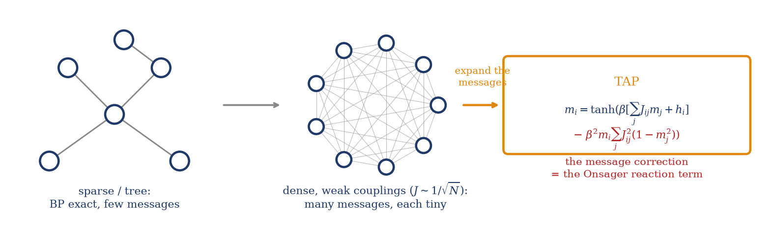
BP contains TAP. The week’s thesis can now be made rigorous. Put belief propagation on the previous lecture’s dense graph — every pair coupled, weakly, \(J \sim 1/\sqrt{N}\) — and expand. For weak bonds the message Equation 12.1 linearizes, \(u_{k\to i} \approx J_{ki}\, m_{k \to i}\), so the marginal reads \(m_i = \tanh(\beta[h_i + \sum_k J_{ki}\, m_{k\to i}])\): naive mean field, except that the inputs are cavity magnetizations. And the cavity magnetization differs from the full one by exactly the neighbor’s linear response to \(i\)’s removal:

\[ m_{k \to i} \;\approx\; m_k \;-\; \underbrace{\beta\big(1 - m_k^2\big)}_{\chi_k}\, J_{ki}\, m_i \qquad\Longrightarrow\qquad m_i = \tanh\!\Big(\beta\Big[ h_i + \sum_k J_{ki} m_k \;-\; \beta\, m_i \sum_k J_{ki}^2 \big(1 - m_k^2\big) \Big]\Big) \]

— the TAP equations Equation 11.3, term for term: the message correction is the Onsager reaction term (Figure 12.2; the systematic \(1/\sqrt N\) bookkeeping is script-level, but the two lines above are the whole idea). The week’s thesis is now a theorem rather than a slogan: message passing is mean-field plus Onsager. On a sparse graph, BP is the richer object — a full message per edge; on a dense one, the many tiny messages collapse and what survives of them, collectively, is precisely the reaction term the previous lecture derived from the Plefka ladder. One idea — the cavity — takes whatever form the graph topology dictates.

Figure 12.2: The week’s thesis, made visual. On a sparse graph (left) belief propagation carries a full message per edge and is exact on trees. Densify the graph — many couplings, each weak, \(J \sim 1/\sqrt{N}\) (center) — and the messages linearize and collapse: expanding the cavity magnetizations to leading order (right) yields exactly the TAP equations, the messages’ collective correction to naive mean field being the Onsager reaction term of Chapter 11. Belief propagation contains TAP; the graph topology chooses the form.

Trap

BP is exact only on trees — and “works” is not “exact.” On loopy graphs, belief propagation may fail to converge, and its fixed points can return wrong marginals: a short loop lets a node’s influence travel around and return as fresh evidence — the self-reaction trees structurally lack (the example below measures the damage growing with the loop’s coupling strength). The Bethe free energy is likewise not a bound off trees. Loopy BP nonetheless works astonishingly often — it is decoding error-correcting codes in your pocket right now — but that is an empirical grace with known failure modes (short loops, strong couplings), not a guarantee. Generalized BP on region graphs (Yedidia, Freeman, and Weiss 2003) repairs loops systematically; we name it here without developing it.

Take-home 2

BP fixed points are stationary points of the Bethe free energy — the pairwise upgrade of Week 5’s functional, exact on trees, with the messages as Lagrange multipliers (Yedidia, Freeman, and Weiss 2003). And on a dense weak-coupling graph the messages collapse: the cavity correction \(m_{k\to i} \approx m_k - \chi_k J_{ki} m_i\) reproduces the TAP equations exactly. Message passing = mean-field + Onsager. On loops, BP is usually excellent and never guaranteed; Bethe is not a bound.

12.5 AMP: TAP for the dense linear model

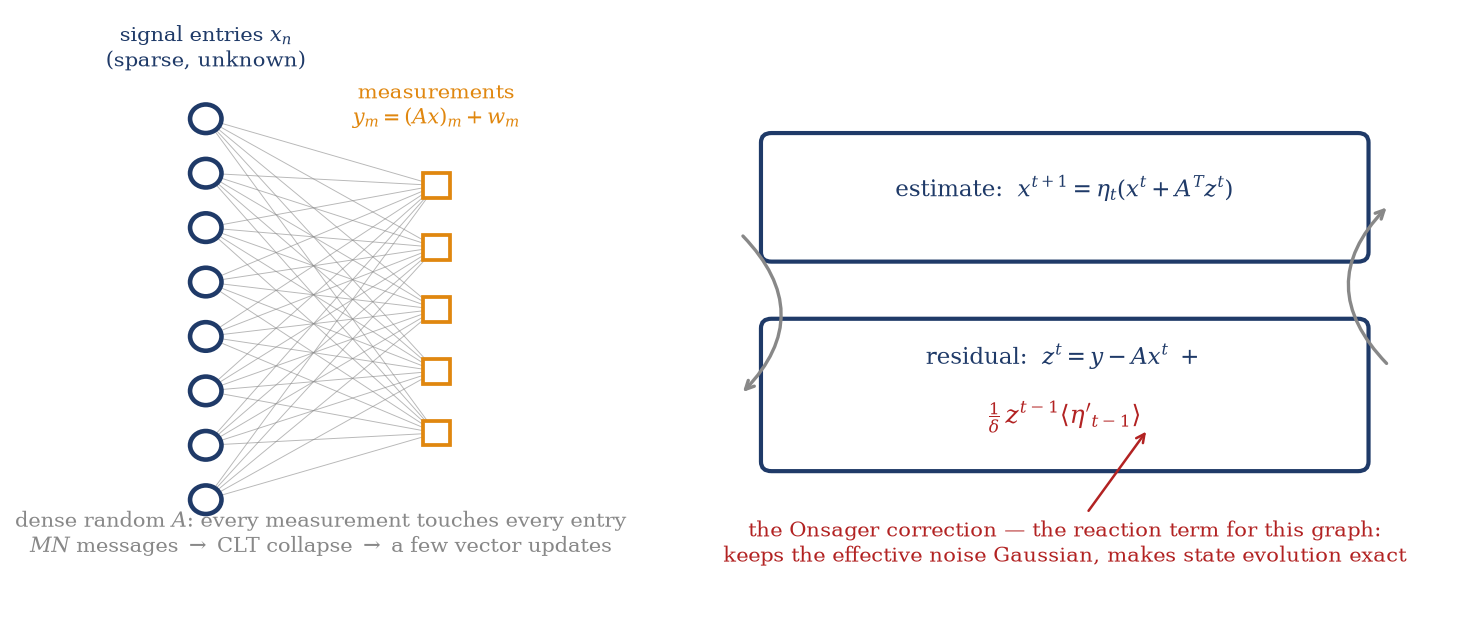
One more graph, chosen because you will derive message passing on it yourselves in the tutorial — and because it is where this fifty-year-old physics became a modern algorithm with a proof. The problem is compressed sensing: observe \(y = A x + w\), with \(A\) an \(M \times N\) dense random matrix (i.i.d. Gaussian entries), \(M < N\) measurements of an \(N\)-dimensional but sparse signal \(x\), noise \(w\). Undersampled linear regression, rescued by sparsity — the workhorse of modern signal recovery (accelerated MRI being the textbook application). As an inference problem it lives on a dense bipartite factor graph (Figure 12.3, left): every measurement touches every signal entry, so literal BP would pass \(2MN\) messages per iteration — computationally impractical, but structurally familiar: a dense graph of weak individual influences, exactly the regime where this lecture just taught you messages collapse.

They do. Because each message is a sum of many weak, nearly independent contributions, the central limit theorem collapses the \(2MN\) messages onto a few vector updates — approximate message passing (Donoho, Maleki, and Montanari 2009). Its structure (stated here; the derivation is deferred to the tutorial): iterate an estimate step, \(x^{t+1} = \eta_t(x^t + A^T z^t)\), where \(\eta_t\) is a scalar denoiser (for sparse signals, a soft-threshold that shrinks small entries to zero), and a residual step,

\[ z^t \;=\; y - A x^t \;+\; \underbrace{\frac{1}{\delta}\, z^{t-1}\, \big\langle \eta_{t-1}' \big\rangle}_{\text{the Onsager correction}}, \qquad \delta = M/N, \]

AMP: the reaction term, again

whose last term is the important one: an extra piece of the residual, proportional to the previous residual and to the average sensitivity \(\langle \eta' \rangle\) of the denoiser — a memory term that naive iterative thresholding does not have. It is called, in the AMP literature and not by coincidence, the Onsager correction term, and its job is the previous lecture’s job: the estimate \(x^t\) was built from the residual, so the naive residual \(y - Ax^t\) is contaminated by the estimate’s own influence reflected back through \(A\) — an echo, through a matrix. Subtracting it decorrelates the effective noise, keeping \(x^t + A^T z^t\) statistically equivalent to signal plus fresh Gaussian noise at every iteration — which is precisely what makes AMP analyzable: a one-dimensional recursion (state evolution) then predicts the algorithm’s error at every step, exactly in the large-system limit. Drop the term and the iteration derails; keep it and the algorithm comes with a proof. The reaction term is not a refinement here — it is the difference between a heuristic and a theorem, exactly as it was the difference between SK’s “solution” and TAP’s.

Two further results connect AMP to the module’s themes. State evolution has a sharp threshold: below a critical measurement rate \(\delta\), recovery fails; above it, in the noiseless limit AMP reconstructs the signal essentially perfectly (with measurement noise the transition is a jump in the reconstruction error rather than to perfection) — a phase transition in an inference problem, the same order-parameter physics that magnetized Week 5’s ferromagnet and collapsed Week 2’s memory, now deciding whether an MRI scan can be undersampled. The derivation of AMP from the collapsing messages, and the full demonstration of how the Onsager correction emerges from the message bookkeeping, are deferred to the tutorial.

Figure 12.3: AMP in one picture. Left: compressed sensing as a graphical model — a dense bipartite graph in which every measurement \(y_m\) touches every unknown signal entry \(x_n\); literal BP would pass \(2MN\) messages, but dense-and-weak is exactly the collapsing regime. Right: the collapsed algorithm (Donoho, Maleki, and Montanari 2009) — an estimate step through a denoiser \(\eta_t\), and a residual step carrying the *Onsager correction* (red): the memory term that subtracts the estimate’‘s own influence reflected back through the measurement matrix, keeps the effective noise Gaussian, and makes the algorithm’’s state-evolution analysis exact. The reaction term of Chapter 11 in signal-processing form — you derive it in the tutorial.

Take-home 3

AMP is belief propagation for the dense compressed-sensing graph, collapsed by the CLT to vector updates — and its residual carries an Onsager correction term that decorrelates the effective noise and makes state evolution exact. Drop it and the iteration fails; keep it and the algorithm has a proof, and a sharp recovery phase transition in the measurement rate. It is TAP for another graphical model.

12.6 Example: exact on the tree, wobbling on the loop, TAP on the dense

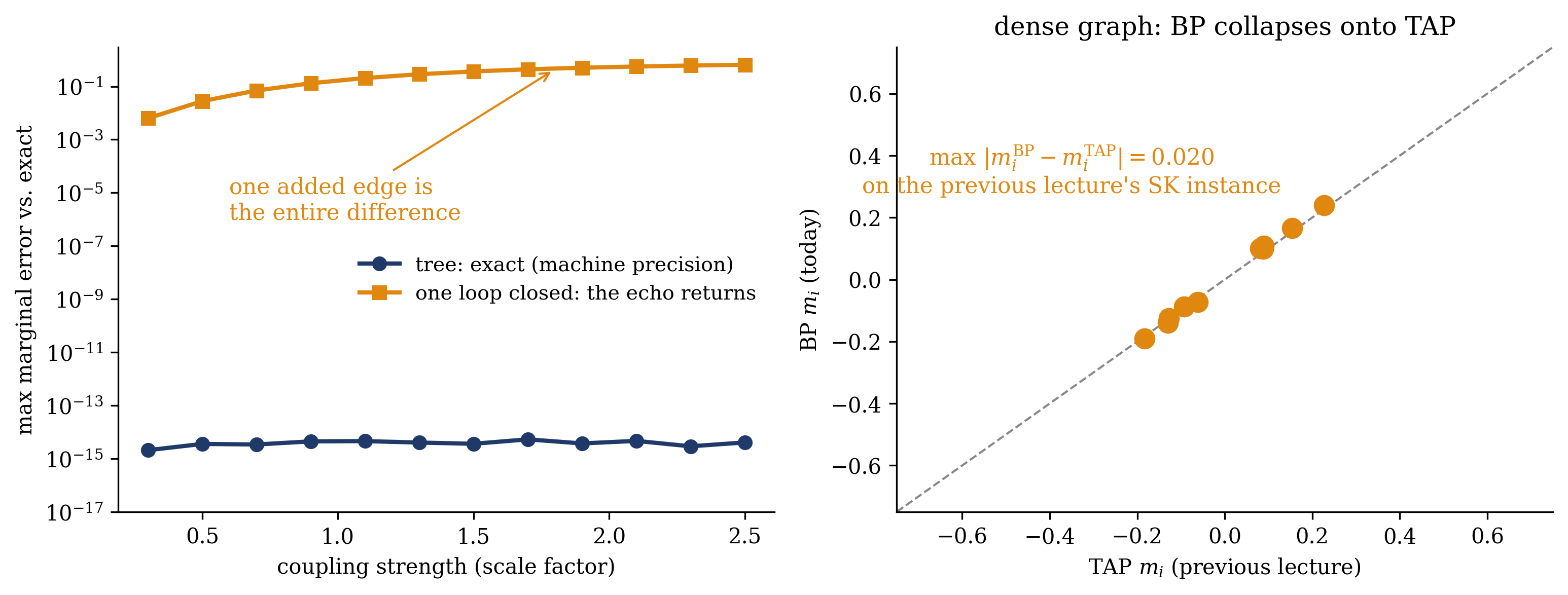
The three claims are tested numerically on three graphs (Figure 12.4). The tree: a seven-node Ising tree with random couplings and fields — BP converges in a handful of sweeps and matches the enumerated marginals to \(4 \times 10^{-15}\): machine precision, the exactness theorem realized numerically. The loop: add one edge to that tree, closing a single cycle, and rerun. BP still converges here, but the marginals are now wrong — by \(0.03\) at weak coupling, growing to \(0.65\) as the loop’s couplings strengthen — while the tree’s error stays at machine zero throughout. One edge is the entire difference, and the mechanism is the one the trap named: around a loop, a node’s influence returns as fake evidence, and the stronger the loop’s couplings, the louder the echo. The dense graph: run full BP on the previous lecture’s SK instance (\(N = 10\), the seed and fields of Section 11.5, \(T = 1.5\)) and set it beside the previous lecture’s TAP solution: the two agree to \(0.02\) across all ten spins — the BP→TAP reduction, verified on the very instance the previous lecture used to test TAP (both, for the record, within \(0.03\) RMS of the enumerated truth).

Show code

def exact_marginals(N, edges, J, h, T):
    S = np.array([[(c >> i & 1) * 2 - 1 for i in range(N)] for c in range(2**N)], dtype=float)
    E = np.zeros(2**N)
    for (a, b), Jab in zip(edges, J):
        E -= Jab * S[:, a] * S[:, b]
    E -= S @ h
    w = np.exp(-(E - E.min()) / T)
    p = w / w.sum()
    return (p[:, None] * S).sum(axis=0)

def bp(N, edges, J, h, T, damp=0.5, iters=5000, tol=1e-14):
    beta = 1.0 / T
    nbrs = {i: [] for i in range(N)}
    for (a, b) in edges:
        nbrs[a].append(b); nbrs[b].append(a)
    u = {(a, b): 0.0 for (a, b) in edges} | {(b, a): 0.0 for (a, b) in edges}
    Jmap = {}
    for (a, b), Jab in zip(edges, J):
        Jmap[(a, b)] = Jmap[(b, a)] = Jab
    for _ in range(iters):
        delta = 0.0
        for (k, i) in u:
            hki = h[k] + sum(u[(l, k)] for l in nbrs[k] if l != i)
            new = (1 / beta) * np.arctanh(np.tanh(beta * Jmap[(k, i)]) * np.tanh(beta * hki))
            delta = max(delta, abs(new - u[(k, i)]))
            u[(k, i)] = (1 - damp) * u[(k, i)] + damp * new
        if delta < tol:
            break
    return np.array([np.tanh((h[i] + sum(u[(k, i)] for k in nbrs[i])) / T) for i in range(N)])

rng = np.random.default_rng(3)
N = 7
tree = [(0, 1), (1, 2), (2, 3), (1, 4), (2, 5), (0, 6)]
J0 = rng.uniform(-1, 1, len(tree))
h0 = rng.normal(0, 0.3, N)
loop = tree + [(3, 5)]
Jl0 = np.append(J0, 0.8)

scales = np.linspace(0.3, 2.5, 12)
err_tree, err_loop = [], []
for c in scales:
    err_tree.append(np.abs(bp(N, tree, c * J0, h0, 1.0)
                           - exact_marginals(N, tree, c * J0, h0, 1.0)).max())
    err_loop.append(np.abs(bp(N, loop, c * Jl0, h0, 1.0)
                           - exact_marginals(N, loop, c * Jl0, h0, 1.0)).max())

fig, (a1, a2) = plt.subplots(1, 2, figsize=(10.4, 4.0))
a1.semilogy(scales, np.maximum(err_tree, 1e-16), "o-", color=NAVY, lw=2,
            label="tree: exact (machine precision)")
a1.semilogy(scales, err_loop, "s-", color=ORANGE, lw=2,
            label="one loop closed: the echo returns")
a1.annotate("one added edge is\nthe entire difference", xy=(1.8, err_loop[7]),
            xytext=(0.6, 1e-6), color=ORANGE, fontsize=10.5,
            arrowprops=dict(arrowstyle="->", color=ORANGE, lw=1))
a1.set_xlabel("coupling strength (scale factor)")
a1.set_ylabel(r"max marginal error vs. exact")
a1.set_ylim(1e-17, 3)
a1.legend(frameon=False, fontsize=9.5, loc="center right")

# dense: BP vs TAP on the W6L1 SK instance
def make_sk(N, Js, seed):
    r = np.random.default_rng(seed)
    Jm = r.normal(0, Js / np.sqrt(N), (N, N)); Jm = (Jm + Jm.T) / np.sqrt(2)
    np.fill_diagonal(Jm, 0.0)
    return Jm, r.normal(0, 0.2, N)

def tap(Jm, h, T, damp=0.3, iters=20000):
    m = np.full(len(h), 0.01); J2 = Jm**2
    for _ in range(iters):
        f = Jm @ m + h - (1 / T) * m * (J2 @ (1 - m**2))
        mn = np.tanh(f / T)
        if np.abs(mn - m).max() < 1e-12:
            return mn
        m = (1 - damp) * m + damp * mn
    return m

N2 = 10
Jm, h2 = make_sk(N2, 1.0, 8)
dense = [(i, j) for i in range(N2) for j in range(i + 1, N2)]
Jd = np.array([Jm[i, j] for (i, j) in dense])
m_bp = bp(N2, dense, Jd, h2, 1.5, damp=0.3, iters=20000)
m_tap = tap(Jm, h2, 1.5)
a2.plot([-1, 1], [-1, 1], color=GRAY, ls="--", lw=1)
a2.plot(m_tap, m_bp, "o", color=ORANGE, ms=9)
a2.text(-0.35, 0.28, rf"max $|m_i^{{\rm BP}} - m_i^{{\rm TAP}}| = {np.abs(m_bp-m_tap).max():.3f}$"
        "\non the previous lecture's SK instance",
        color=ORANGE, fontsize=10.5, ha="center")
a2.set_xlabel(r"TAP $m_i$ (previous lecture)"); a2.set_ylabel(r"BP $m_i$ (today)")
a2.set_title("dense graph: BP collapses onto TAP", fontsize=12)
a2.set_xlim(-0.75, 0.75); a2.set_ylim(-0.75, 0.75)
fig.tight_layout(); plt.show()

Figure 12.4: The lecture’s three claims, run. Left: maximum marginal error of BP against exact enumeration, versus the strength of the couplings, on a seven-node tree (navy — flat at machine precision, \(\sim 10^{-15}\): the exactness theorem) and on the same graph with *one* added edge closing a single loop (orange — the error grows from \(0.006\) to \(0.65\) as the loop’s couplings strengthen: influence returning around the cycle, the self-reaction trees lack). Right: on the dense graph, BP collapses onto TAP — the BP marginals of the previous lecture’s \(N = 10\) SK instance (Section 11.5, same seed, \(T = 1.5\)) against the previous lecture’s TAP solution, on the diagonal to within \(0.02\). One idea, three graphs: exact where removal disconnects, echoing where it does not, and TAP where the graph is dense.

The cavity field is a message; passed on a tree it is exact, passed on a dense graph it is TAP — message passing is mean-field plus Onsager.

The tutorial (16–18, Ph12 106) is derivation-led. Two problems, both applications of today’s machinery: run belief propagation on a specific Ising tree by hand and check it against the exact answer, then derive approximate message passing for compressed sensing from the collapsing messages.

12.7 Outlook: the week’s thesis, complete

Week 6 closes with a single idea spanning four apparently different objects. The previous lecture derived one term — the Onsager reaction, a spin’s self-echo subtracted from its effective field — twice, and found its size governed by \(\sum_j J_{ij}^2\). Today the same cavity idea, run recursively, became an algorithm: exact on trees, variational through the Bethe free energy, and collapsing — on dense graphs — back onto the previous lecture’s equations, the messages’ correction being the reaction term. In the tutorial it becomes a second algorithm, on a second graph, with the same term reappearing in a residual update and earning, this time, an exactness proof. Mean field, TAP, belief propagation, and AMP are one idea at four levels of graph structure, with a progressively weaker set of guarantees — a bound (W5), an estimate (TAP), tree-exactness (BP), asymptotic exactness with state evolution (AMP) — each relaxed in exchange for broader applicability.

The two routes through disordered systems can now be compared. Week 2 introduced the replica method’s results; the previous lecture presented the cavity route as the alternative. The cavity route is the one that became algorithms: belief propagation decodes the LDPC codes in every modern radio (Gallager 1962), and AMP reconstructs undersampled signals with performance guarantees (Donoho, Maleki, and Montanari 2009). The cavity method is how disordered-systems physics entered algorithm design.

The module now turns toward machine learning proper. Week 7 takes the variational thread to its ML destination: latent-variable models, the auxiliary-field (Hubbard–Stratonovich) trick for manufacturing latents, and the variational autoencoder — where Week 5’s ELBO stops being a physicist’s identity and becomes the literal training loss of a deep generative network, with Week 5’s reverse-KL warnings manifesting as posterior collapse. After that, Module 3 finally takes the other road out of the intractable \(Z\) — not approximating the distribution but sampling it — and the two roads will meet again in Module 4, where \(Z\) is neither approximated nor sampled but removed from the objective altogether.