14 The variational autoencoder: minimizing free energy by backpropagation

14.1 The objective we already have

Module 2 ends with a trainable model. The previous lecture closed the circle it had opened: a latent-variable model \(p_\theta(x) = \int \mathrm{d}z\, p(z)\, p_\theta(x \mid z)\) is an interacting system with the interaction integrated out — the latent \(z\) is a decoupling field (Section 13.4) — and learning such a model runs immediately into the posterior \(p_\theta(z \mid x)\), which is intractable for the same reason \(Z\) always was. Week 5 told us what to do about that: replace the posterior by a tractable \(q\), and optimize the evidence lower bound, which is nothing but the negative variational free energy (Equation 9.2). So the objective is settled. What is not settled is whether anyone can train it. Between the ELBO on the blackboard and a generative model fitted to a million images stand two concrete obstacles, and today’s lecture is the removal of both.

The first obstacle is bookkeeping that does not scale. Classical variational inference — and its ancestor, the EM algorithm — optimizes a separate variational distribution \(q\) for every data point: one free-standing optimization per image, re-run from scratch for any image not seen before. The second obstacle is a gradient that does not exist where we need it. The ELBO is an expectation over \(q_\phi(z \mid x)\), and its parameters \(\phi\) sit inside the distribution being sampled; back-propagation, which differentiates compositions of deterministic functions, cannot pass through the random draw of a \(z\).

In 2014 both obstacles fell at once, twice. Kingma and Welling (2014) and, independently and nearly simultaneously, Rezende, Mohamed, and Wierstra (2014) proposed the same pair of fixes: replace the per-datapoint \(q\) by a single neural network — an encoder — that outputs the variational parameters for any \(x\) in one forward pass, and rewrite the random draw as a deterministic, differentiable function of the parameters plus external noise. The resulting model, the variational autoencoder (VAE), launched deep generative modeling as a field. Its lineage is worth a sentence: the idea of pairing a recognition network with a generative network and training them together is the Helmholtz machine of Dayan et al. (1995) — a name chosen, twenty years before this course, precisely because the objective being optimized is a free energy.

The driving question of the lecture: how do you train Week 5’s free-energy minimization on a dataset too large to enumerate and a model too deep to solve?

Take-home 1

The ELBO (\(= -F_\mathrm{var}\), Week 5) is the right objective for a latent-variable model, but two obstacles block training it at scale: classical VI optimizes a fresh \(q\) per data point, and the gradient in the variational parameters cannot pass through a random sample. The VAE (Kingma and Welling 2014; Rezende, Mohamed, and Wierstra 2014) removes both — amortized inference (one encoder network for all data) and the reparameterization trick (a differentiable sampler) — turning free-energy minimization into a network trained by SGD.

14.2 Two obstacles, two fixes

The structure is a two-by-two correspondence, worth stating before any formula. Obstacle one, per-datapoint inference, is removed by amortization: a single network \(q_\phi(z \mid x)\) learns the map from data to variational parameters, so that inference on a new \(x\) costs one forward pass rather than one optimization. Obstacle two, non-differentiable sampling, is removed by reparameterization: the sample \(z\) is rewritten as a deterministic function of \(\phi\) and a parameter-free noise \(\varepsilon\), so that gradients flow through the sampler like through any other layer. The first provides scale; the second provides gradients; together they make the ELBO an objective like any other in deep learning — evaluated on minibatches, differentiated by backprop, optimized by SGD.

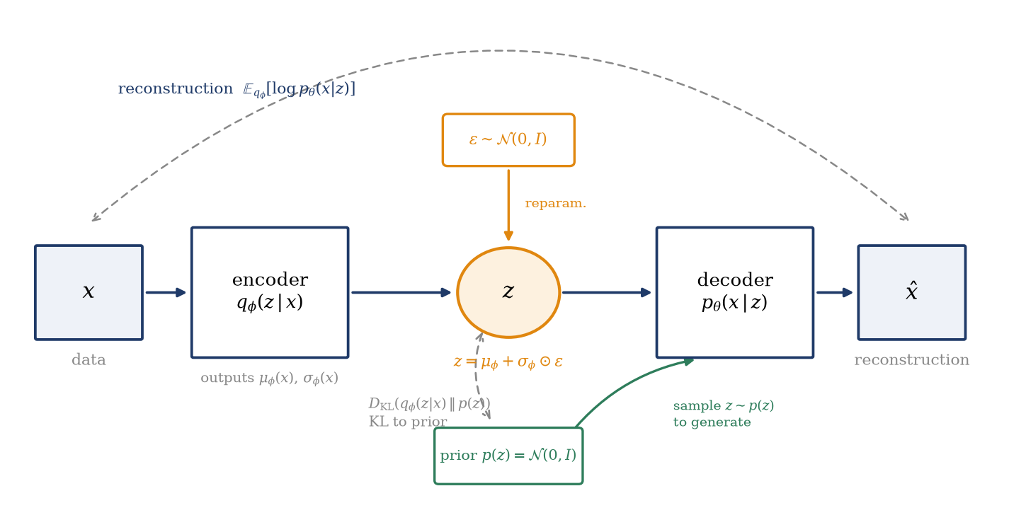
Figure 14.1 assembles the machine these fixes produce, and everything that follows is a derivation of one of its parts. Data \(x\) enters the encoder \(q_\phi(z \mid x)\), which outputs the mean \(\mu_\phi(x)\) and standard deviation \(\sigma_\phi(x)\) of a Gaussian over the latent; a sample \(z = \mu_\phi + \sigma_\phi \odot \varepsilon\) is drawn with external noise \(\varepsilon\) (\(\odot\) is the elementwise product); the decoder \(p_\theta(x \mid z)\) maps the latent back to a distribution over data space, scored against the input. Two terms tie the loop together: the reconstruction term compares the decoder’s output to \(x\), and a KL term holds the encoder’s distribution near the prior \(p(z) = \mathcal{N}(0, I)\). That KL term is what separates this machine from a plain autoencoder, and the distinction is the whole point: because every encoder output is pulled toward the same prior, a \(z\) drawn from that prior is a legitimate input to the decoder — the model can generate, not only compress. A deterministic autoencoder has no prior to sample from and cannot.

Figure 14.1: The central picture of the lecture: the variational autoencoder. Data \(x\) enters the encoder \(q_\phi(z \mid x)\), which outputs the variational parameters \(\mu_\phi(x), \sigma_\phi(x)\); the latent is sampled through the reparameterization \(z = \mu_\phi + \sigma_\phi \odot \varepsilon\) with external noise \(\varepsilon \sim \mathcal{N}(0, I)\) (orange), and the decoder \(p_\theta(x \mid z)\) scores the reconstruction against the input. The two loss terms are drawn in gray: the reconstruction term (top) compares \(\hat{x}\) to \(x\); the KL term (bottom) holds the encoder near the prior \(p(z) = \mathcal{N}(0, I)\). Generation (green) bypasses the encoder entirely: sample \(z \sim p(z)\) and decode.

One notational flag before the derivations, because two parameter sets now live in one objective. Throughout, \(\theta\) denotes the decoder (generative) parameters and \(\phi\) the encoder (inference) parameters; the ELBO is optimized over both, but the two gradients raise entirely different issues — \(\nabla_\theta\) is routine, and \(\nabla_\phi\) is the subject of Section 14.4. The latent \(z\) is the previous lecture’s auxiliary field (Chapter 13), here continuous and Gaussian; \(\varepsilon\) is the reparameterization noise, not an energy scale. And we work at \(T = 1\) with the manufactured energy \(E(z) = -\log p_\theta(x, z)\) of Section 9.4, so the machine-learning literature’s \(\mathbb{E}_{q_\phi}[\,\cdot\,]\) is our \(\langle \cdot \rangle_{q_\phi}\); we keep the course’s angle brackets.

14.3 The engine, part I: two terms, one encoder

The ELBO as Week 5 left it is one number — a lower bound on the log-evidence. To train a network we need it in the two pieces the network will trade off, and the split takes four lines. Start from the master identity, Equation 9.2, specialized to an \(x\)-dependent variational family:

\[ \log p_\theta(x) \;=\; \mathrm{ELBO}(\theta, \phi; x) \;+\; D_\mathrm{KL}\big(q_\phi(z \mid x) \,\big\|\, p_\theta(z \mid x)\big), \qquad \mathrm{ELBO} \;=\; \big\langle \log p_\theta(x, z) \big\rangle_{q_\phi} - \big\langle \log q_\phi(z \mid x) \big\rangle_{q_\phi}. \]

Since the gap on the right is a KL divergence, it is non-negative, and the ELBO bounds the evidence from below — that much is Week 5 verbatim. Now split the joint along the generative structure of Equation 13.4, \(p_\theta(x, z) = p(z)\, p_\theta(x \mid z)\), and regroup:

\[ \mathrm{ELBO} \;=\; \big\langle \log p_\theta(x \mid z) \big\rangle_{q_\phi} + \big\langle \log p(z) \big\rangle_{q_\phi} - \big\langle \log q_\phi(z \mid x) \big\rangle_{q_\phi} \;=\; \big\langle \log p_\theta(x \mid z) \big\rangle_{q_\phi} - \Big\langle \log \frac{q_\phi(z \mid x)}{p(z)} \Big\rangle_{q_\phi}, \]

and the last average is again a KL divergence — this time between the encoder and the prior:

\[ \boxed{\; \mathrm{ELBO}(\theta, \phi; x) \;=\; \underbrace{\big\langle \log p_\theta(x \mid z) \big\rangle_{q_\phi(z \mid x)}}_{\text{reconstruction}} \;-\; \underbrace{D_\mathrm{KL}\big(q_\phi(z \mid x) \,\big\|\, p(z)\big)}_{\text{KL to prior}} \;} \tag{14.1}\]

ELBO decomposition

The two terms pull against each other, and their tension is the model. The reconstruction term is the log-likelihood the decoder assigns to the data given its inferred latent: it grows when \(z\) carries information about \(x\), so it pushes the encoder to be informative. The KL regularizer measures how far the encoder strays from the prior: it shrinks when \(z\) carries nothing, so it pushes the encoder to be forgettable. A trained VAE sits where the two forces balance — enough structure in the latent to reconstruct, little enough to keep the latent space close to the prior it must share with generation. And by Week 5’s identity, the whole expression is \(-F_\mathrm{var}(q_\phi)\): reconstruction plays the energy term, the KL plays the entropy-and-prior term, and we will make that mapping exact in Section 14.6 once the objective is trainable.

Amortization. As it stands, Equation 14.1 still expects a separate \(q\) per data point: classical variational inference would now optimize the variational parameters of \(q\) for this \(x\), then start over for the next one. For a dataset of \(10^5\) images that is \(10^5\) optimizations per gradient step, and for a test image it is one more. The fix is to make the variational parameters a function of \(x\) and learn the function once:

\[ q_\phi(z \mid x) \;=\; \mathcal{N}\!\big(z;\; \mu_\phi(x),\; \mathrm{diag}\,\sigma_\phi^2(x)\big), \tag{14.2}\]

amortized Gaussian encoder

where \(\mu_\phi(x)\) and \(\sigma_\phi(x)\) are the outputs of one neural network with weights \(\phi\). This is amortized inference: the cost of inference is paid once, during training, and thereafter every data point — including data never seen — gets its approximate posterior in a single forward pass. The trade-off is explicit. A single network cannot match the optimal per-datapoint \(q\) on every \(x\), so the amortized ELBO sits below what classical VI could reach; that shortfall is the amortization gap, distinct from the approximation gap \(D_\mathrm{KL}(q_\phi \| p_\theta(z \mid x))\) that any restricted family pays. The two gaps stack — the family’s first, then the function’s — and both reappear in the traps below.

The objective now scales, but it is not yet differentiable where it matters: the reconstruction term is an average over \(q_\phi(z \mid x)\), and training the encoder needs \(\nabla_\phi\) of that average. That gradient is the subject of the next section.

14.4 The engine, part II: the reparameterization trick

The problem, stated precisely: we need \(\nabla_\phi \langle f(z) \rangle_{q_\phi}\), the gradient of an expectation with respect to the parameters of the distribution being averaged over. Backprop differentiates deterministic compositions; a sample \(z \sim q_\phi\) is not one. There is a classical estimator for exactly this object, and its failure is what makes the trick necessary. Differentiate the integral directly and insert \(\nabla_\phi q_\phi = q_\phi \nabla_\phi \log q_\phi\):

\[ \nabla_\phi \big\langle f(z) \big\rangle_{q_\phi} \;=\; \int \mathrm{d}z\, f(z)\, \nabla_\phi q_\phi(z \mid x) \;=\; \big\langle f(z)\, \nabla_\phi \log q_\phi(z \mid x) \big\rangle_{q_\phi}. \]

This is the score-function (or REINFORCE) estimator: unbiased, universal — it never differentiates \(f\), so \(f\) may be a black box — and, for our purposes, uselessly noisy. The reason is structural: the estimator multiplies the value of \(f\) by the score, so its fluctuations track the magnitude of \(f\) across the whole distribution rather than the local sensitivity of \(f\) to \(\phi\); every irrelevant fluctuation of \(f\) enters at full strength. Baselines and control variates tame it somewhat, but the variance grows with the dimension of \(z\) (the example below measures the growth), and deep latent models sit exactly where it hurts.

The reparameterization trick replaces value-times-score by an actual derivative. For the Gaussian encoder of Equation 14.2, write the sample as a deterministic map applied to parameter-free noise:

\[ \boxed{\; z \;=\; \mu_\phi(x) + \sigma_\phi(x) \odot \varepsilon, \qquad \varepsilon \sim \mathcal{N}(0, I), \;} \tag{14.3}\]

reparameterization trick

which leaves the distribution of \(z\) unchanged but relocates the randomness: the expectation is now over a fixed distribution, and the parameters sit inside the integrand, where \(\nabla_\phi\) can reach them,

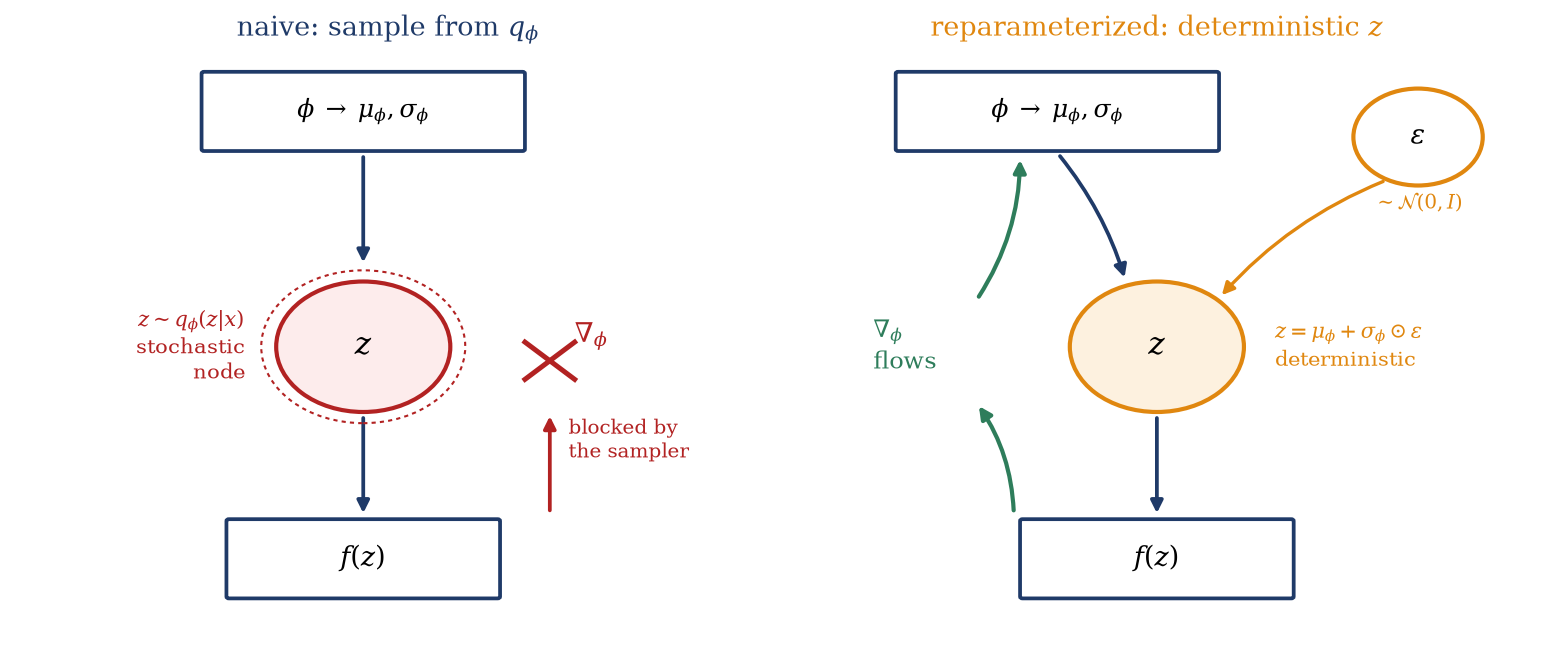
\[ \big\langle f(z) \big\rangle_{q_\phi} = \big\langle f\big(\mu_\phi + \sigma_\phi \odot \varepsilon\big) \big\rangle_{\varepsilon}, \qquad \nabla_\phi \big\langle f(z) \big\rangle_{q_\phi} = \Big\langle \nabla_z f\big(z\big) \cdot \nabla_\phi \big(\mu_\phi + \sigma_\phi \odot \varepsilon\big) \Big\rangle_{\varepsilon}. \]

The sampler has become a differentiable layer (Figure 14.2): forward, draw \(\varepsilon\) and compute \(z\); backward, gradients flow through \(\mu_\phi\) and \(\sigma_\phi\) by the chain rule, exactly as through any affine layer with an input. This pathwise gradient uses \(\nabla_z f\) — the local slope, not the global value — and its variance is correspondingly small; one draw of \(\varepsilon\) per data point is standard practice and usually enough. The trick does demand something in return: the latent must admit such a deterministic-map-plus-fixed-noise form, which continuous families do and discrete ones do not — for discrete latents one falls back on score-function estimators or the Gumbel-softmax relaxation, which we name and set aside.

Figure 14.2: The enabling idea as two computation graphs. Left: sampling \(z\) directly from \(q_\phi(z \mid x)\) makes \(z\) a stochastic node, and the backward pass cannot cross it — the gradient in \(\phi\) is blocked at the sampler. Right: the reparameterized graph. The noise \(\varepsilon \sim \mathcal{N}(0, I)\) enters as an input, \(z = \mu_\phi + \sigma_\phi \odot \varepsilon\) is a deterministic node, and \(\nabla_\phi\) flows from \(f(z)\) back through \(\mu_\phi, \sigma_\phi\) (green) by ordinary backpropagation.

The KL term costs nothing. The second term of Equation 14.1 needs no estimator at all: for a Gaussian encoder against the standard-normal prior it is a closed-form function of the encoder outputs. Per latent dimension, with \(q = \mathcal{N}(\mu, \sigma^2)\) and \(p = \mathcal{N}(0, 1)\),

\[ D_\mathrm{KL}(q \,\|\, p) = \Big\langle \log \frac{q(z)}{p(z)} \Big\rangle_q = \Big\langle -\frac{(z - \mu)^2}{2\sigma^2} + \frac{z^2}{2} - \log \sigma \Big\rangle_q = \frac{1}{2}\big( \mu^2 + \sigma^2 - 1 - \log \sigma^2 \big), \]

using \(\langle (z-\mu)^2 \rangle_q = \sigma^2\) and \(\langle z^2 \rangle_q = \mu^2 + \sigma^2\). Summed over dimensions:

\[ D_\mathrm{KL}\big(q_\phi(z \mid x) \,\big\|\, \mathcal{N}(0, I)\big) \;=\; \frac{1}{2} \sum_j \Big( \mu_j^2 + \sigma_j^2 - 1 - \log \sigma_j^2 \Big). \tag{14.4}\]

Gaussian KL, closed form

Assemble the objective. Estimate the reconstruction term by Monte Carlo over \(\varepsilon\) — a single draw per data point — take the KL in closed form, and average over a minibatch:

\[ \mathcal{L}(\theta, \phi) \;=\; \frac{1}{N} \sum_{x} \Big[ \log p_\theta\big(x \,\big|\, \mu_\phi(x) + \sigma_\phi(x) \odot \varepsilon\big) \;-\; D_\mathrm{KL}\big(q_\phi(z \mid x) \,\big\|\, p(z)\big) \Big], \tag{14.5}\]

VAE training objective

maximized over \((\theta, \phi)\) jointly by SGD. The form of the reconstruction term follows from the decoder’s likelihood: a Bernoulli decoder (binarized MNIST, the tutorial) makes it a binary cross-entropy, a Gaussian decoder makes it a mean-squared error up to constants — the standard losses of supervised learning, reappearing as likelihood choices. Trained, the network is two machines in one: a generative model (draw \(z \sim \mathcal{N}(0, I)\), decode) and a representation learner (encode \(x\), keep \(z\)). Amortization made the objective scale; reparameterization made it differentiable; with both, Week 5’s free-energy minimization is a network trained by gradient descent.

Take-home 2

The score-function estimator \(\langle f \nabla_\phi \log q_\phi \rangle\) is unbiased but tracks the value of \(f\), and its variance grows with latent dimension. The reparameterization trick \(z = \mu_\phi + \sigma_\phi \odot \varepsilon\), \(\varepsilon \sim \mathcal{N}(0, I)\), moves the randomness onto a fixed distribution so the gradient uses the slope \(\nabla_z f\) instead — low variance, one noise draw per data point. With the closed-form Gaussian KL (Equation 14.4), the VAE objective (Equation 14.5) trains by ordinary SGD.

14.5 Example: two estimators of one gradient

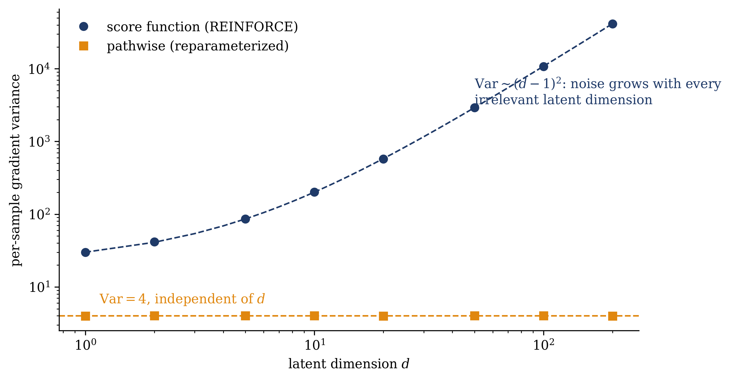
The variance claim can be made quantitative on a toy example. Take \(f(z) = \|z\|^2\) in \(d\) latent dimensions, \(q_\phi = \mathcal{N}(\mu, I)\) with \(\mu = (1, 0, \dots, 0)\), and estimate one gradient component, \(\partial_{\mu_1} \langle f \rangle = 2\mu_1 = 2\) — known exactly, so every estimator can be judged against the truth. Both estimators are unbiased; the question is their spread over single samples. A short calculation with Gaussian moments (worth doing once by hand) gives, per sample,

\[ \mathrm{Var}\big[\hat{g}_\text{score}\big] = (d - 1)^2 + 10\,(d - 1) + 30, \qquad \mathrm{Var}\big[\hat{g}_\text{pathwise}\big] = 4 : \]

the pathwise variance is independent of dimension — the estimator \(2 z_1\) never sees the other \(d - 1\) coordinates — while the score-function estimator multiplies the full value \(\|z\|^2\), fluctuations of every irrelevant dimension included, by the score of \(z_1\), and its variance grows quadratically with \(d\). Figure 14.3 samples both. Already at \(d = 2\) the score-function estimator is ten times noisier (\(41\) against \(4\)); at \(d = 100\) its variance is \(1.08 \times 10^4\), a factor \(2{,}700\) above pathwise, and a latent of realistic size would need thousands of samples to match what reparameterization delivers with one. Figure 14.3 summarizes the case: at realistic latent dimensions, reparameterization reduces the variance by orders of magnitude, making training feasible with a single noise draw per data point.

Show code

rng = np.random.default_rng(7)
dims = np.array([1, 2, 5, 10, 20, 50, 100, 200])
n_samp = 200_000
var_sf, var_pw = [], []
for d in dims:
    eps = rng.standard_normal((n_samp, d))
    z = eps.copy()
    z[:, 0] += 1.0                        # mu = (1, 0, ..., 0), sigma = 1
    f = (z**2).sum(axis=1)
    g_score = f * eps[:, 0]               # f(z) * d(log q)/d(mu_1)
    g_path = 2 * z[:, 0]                  # d(f)/d(z_1) * d(z_1)/d(mu_1)
    var_sf.append(g_score.var())
    var_pw.append(g_path.var())

fig, ax = plt.subplots(figsize=(8.0, 4.2))
ax.loglog(dims, var_sf, "o", color=NAVY, ms=6, label="score function (REINFORCE)")
ax.loglog(dims, var_pw, "s", color=ORANGE, ms=6, label="pathwise (reparameterized)")
dd = np.linspace(1, 200, 200)
ax.loglog(dd, (dd - 1)**2 + 10 * (dd - 1) + 30, ls="--", lw=1.2, color=NAVY)
ax.axhline(4, ls="--", lw=1.2, color=ORANGE)
ax.annotate(r"$\mathrm{Var} \sim (d-1)^2$: noise grows with every"
            "\nirrelevant latent dimension",
            xy=(50, 3.3e3), fontsize=10, color=NAVY, ha="left")
ax.text(1.15, 6.0, r"$\mathrm{Var} = 4$, independent of $d$", fontsize=10, color=ORANGE)
ax.set_xlabel(r"latent dimension $d$")
ax.set_ylabel("per-sample gradient variance")
ax.legend(frameon=False, fontsize=10, loc="upper left")
fig.tight_layout(); plt.show()

Figure 14.3: One gradient, two estimators: the per-sample variance of \(\partial_{\mu_1}\langle\, \|z\|^2 \rangle_{q}\) for \(q = \mathcal{N}(\mu, I)\), \(\mu = (1, 0, \dots, 0)\), as a function of the latent dimension \(d\) (\(2 \times 10^5\) samples per point; dashed lines are the exact Gaussian-moment results). The score-function estimator \(\|z\|^2 (z_1 - \mu_1)\) (navy) multiplies the full value of \(f\) — every irrelevant dimension’s fluctuation included — by the score, and its variance grows as \((d-1)^2\): at \(d = 100\) it reaches \(1.08 \times 10^4\). The pathwise (reparameterized) estimator \(2 z_1\) (orange) uses the slope of \(f\) and stays at \(4\), independent of dimension — a factor \(2{,}700\) below score-function at \(d = 100\). Both estimators are unbiased; only one is trainable.

14.6 What we trained, in Week 5’s language

The correspondence with Week 5 is now direct. Fix a data point \(x\) and manufacture the energy of Section 9.4, \(E(z) = -\log p_\theta(x, z)\) at \(T = 1\); then the variational free energy of the encoder is

\[ F_\mathrm{var}(q_\phi) \;=\; \langle E \rangle_{q_\phi} - S[q_\phi] \;=\; -\underbrace{\big\langle \log p_\theta(x \mid z) \big\rangle_{q_\phi}}_{\text{reconstruction} \;=\; -\langle E \rangle \text{ (data term)}} \;+\; \underbrace{D_\mathrm{KL}\big(q_\phi(z \mid x) \,\big\|\, p(z)\big)}_{\text{KL to prior} \;=\; \text{entropy/prior term}} \;=\; -\,\mathrm{ELBO}, \tag{14.6}\]

the VAE loss is the variational free energy

term for term: the reconstruction plays the energy, the KL regularizer bundles the entropy of \(q_\phi\) with the prior, and the training loss \(-\mathcal{L}\) of Equation 14.5 is \(F_\mathrm{var}\) averaged over the dataset. Training a VAE is variational free-energy minimization with an amortized, neural \(q\) — the physicist minimizing \(F_\mathrm{var}\) over a trial family and the engineer running Equation 14.5 through an optimizer are performing the same optimization on the same functional. The tutorial trains a small VAE on MNIST and tracks reconstruction and KL individually over training.

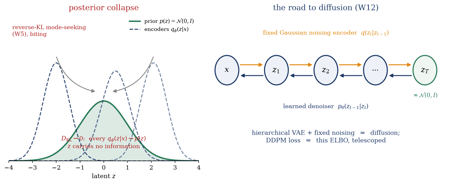
Posterior collapse. Week 5 flagged that variational inference minimizes the reverse KL and warned that its mode-seeking, variance-underestimating character would return (Figure 9.3); here the consequence becomes concrete. Suppose the decoder is expressive enough to model the data with no help from the latent — an autoregressive decoder on images can be. Then the reconstruction term no longer needs \(z\), the KL term is unopposed, and the optimum drives \(q_\phi(z \mid x) \to p(z)\) for every \(x\): the KL reaches zero, the latent carries no information, and the “generative model” degenerates into a decoder that ignores its own code (Figure 14.4, left). This is posterior collapse, the VAE’s characteristic failure, and it is Week 5’s zero-forcing made concrete — the reverse KL pays nothing for abandoning latent structure the decoder can fake. The standard fixes reweight the balance: the β-VAE of Higgins et al. (2017) multiplies the KL term by a coefficient β (a KL weight — not an inverse temperature, despite this course’s reflexes), KL annealing ramps that weight from zero during training, and free bits exempt a per-dimension quota of KL from the loss. Each adjusts the same balance between reconstruction sharpness and latent structure.

Where the intractability went. Placing the VAE alongside Module 1’s models clarifies the comparison. The RBM (Chapter 6) is an undirected model: its \(Z\) runs over all configurations, the likelihood gradient needs the model average (Equation 5.5), and Week 3 dodged it by sampling a little and accepting CD’s bias. The VAE is a directed model: the decoder conditional \(p_\theta(x \mid z)\) is normalized by construction and the prior is fixed, so there is no \(Z\) over \(x\) to fight — the hard object is now the posterior \(p_\theta(z \mid x)\), and the encoder approximates it variationally. The intractability was moved, not removed, and identifying where it sits in each model family is a useful organizing principle: undirected models pay at the partition function, directed models pay at the posterior, and every generative-modeling method in this course is a choice of where to pay.

Trap

Two KLs, one bound, and one trick leave three ways to slip. ① The ELBO’s own KL term is \(D_\mathrm{KL}(q_\phi(z \mid x) \| p(z))\) — encoder to prior, the regularizer inside the objective. The ELBO’s gap is \(D_\mathrm{KL}(q_\phi(z \mid x) \| p_\theta(z \mid x))\) — encoder to posterior, the distance to the evidence. Conflating them is the classic error; only the first is computable, and only the second measures approximation quality. ② The ELBO is a lower bound, not the likelihood: a trained VAE sits below its own model’s \(\log p_\theta(x)\) by the approximation gap plus the amortization gap. ③ The reparameterization trick requires a latent that is a differentiable transform of fixed noise — Gaussians qualify, discrete latents do not (Gumbel-softmax or score-function methods take over there).

Take-home 3

The VAE loss is \(F_\mathrm{var}\) (Equation 14.6): reconstruction is the data/energy term, the KL to the prior is the entropy/prior term, and training is amortized variational free-energy minimization. Its signature failure, posterior collapse — the KL unopposed, the latent ignored — is Week 5’s reverse-KL zero-forcing in practice; β-VAE, KL annealing, and free bits reweight the balance. Keep the two KLs straight: the regularizer points at the prior, the gap points at the posterior.

The VAE is Week 5’s variational free energy, minimized by a neural network — reconstruction against a KL regularizer.

14.7 Outlook: the tutorial, and the road to diffusion

Module 2 set out to approximate an intractable distribution and found four ways to do it: the factorized family (Week 5), the corrected expansion (Chapter 11), message passing on the graph (Chapter 12), and the decoupled latent-variable model (this week). The unifying result is that all four optimize the same functional — the variational free energy — over different families, and that the last of them is not an approximation scheme at all but a model class, trained by descending that functional with a neural network. The tutorial (16–18, Ph12 106) makes the claim concrete: training a small VAE on binarized MNIST, inspecting reconstructions, prior samples, and a two-dimensional latent space, and decomposing the trained ELBO into its two terms. It is one of the computation-led weeks, so the training runs on the groups’ own machines after the predictions are written down.

The connection to the course’s title is direct. A VAE has one latent layer; nothing forbids a hierarchy, \(x \to z_1 \to \dots \to z_T\), each layer conditioned on the last. Now make one deliberately strange choice: fix the encoder to a chain of Gaussian noising steps \(q(z_t \mid z_{t-1})\) — no parameters, no learning, just incremental corruption of the data toward \(z_T \approx \mathcal{N}(0, I)\) — and learn only the decoder chain \(p_\theta(z_{t-1} \mid z_t)\) that runs the corruption backwards (Figure 14.4, right). That model is a diffusion model, and its training loss — the DDPM objective of Week 12 (Ho, Jain, and Abbeel 2020; Sohl-Dickstein et al. 2015) — is this lecture’s ELBO, telescoped along the hierarchy into a sum of per-step denoising terms. The free energy that entered the course as a bound in Week 5 and became a training objective today will train the generative models of Module 4 unchanged; from Boltzmann to diffusion is, at the level of the objective, one equation carried forward.

Figure 14.4: Left: posterior collapse. A powerful decoder leaves the KL term unopposed, and every encoder distribution \(q_\phi(z \mid x)\) (navy, dashed) is driven onto the prior \(p(z)\) (green): the KL reaches zero and the latent carries no information — Week 5’s reverse-KL zero-forcing in practice. Right: the road to diffusion. Stack latents \(x \to z_1 \to \dots \to z_T\) with a *fixed* Gaussian noising encoder (orange) and a learned denoising decoder (navy): a hierarchical VAE whose ELBO, telescoped over the steps, is the DDPM training loss of Week 12.

Every method since Week 5 has approximated or transformed the distribution; none has drawn from it. Module 3 takes the complementary approach and samples: Monte Carlo and the Metropolis rule, annealing on rugged landscapes, and stochastic gradient descent read as a Langevin process — the machinery that turns Week 2’s energy landscapes and this module’s free energies into working algorithms.