16 Simulated annealing: optimization by cooling

16.1 Temperature becomes an instrument

The previous lecture’s Metropolis chain has one parameter. The Metropolis chain samples \(p \propto e^{-E/T}\) at whatever temperature we choose, using only energy differences, and its cost is mixing: the autocorrelation time \(\tau\) that diverges at critical points and grows exponentially in glassy landscapes. Throughout that lecture the knob stayed fixed — temperature was part of the problem statement, the \(T\) at which we wanted equilibrium averages. Today we turn it while the chain runs. Hot, the walker of Figure 15.2 ignores barriers and roams the whole landscape; cold, it commits to a basin and refines downhill. Start hot and cool slowly, and the chain rides the Boltzmann distribution’s own concentration onto low-energy states all the way down to the ground state. A sampler, cooled, becomes an optimizer — that is simulated annealing, and it is Module 3’s second theme: the dynamics of the sampler as a subject in itself.

The name is not a metaphor; it is a lab procedure. A metallurgist who wants a defect-free crystal — the global minimum of the lattice energy — heats the metal and cools it slowly, so that at every stage the atoms stay near thermal equilibrium and settle collectively into ever-lower-energy arrangements. Cool the same melt fast — a quench — and it freezes wherever it happens to be: a glass, disordered, trapped in a local minimum of the energy, held there by barriers it no longer has the thermal energy to cross. In 1983 Kirkpatrick, Gelatt, and Vecchi took this procedure literally (Kirkpatrick, Gelatt, and Vecchi 1983): replace the metal’s energy by any cost function, the atoms’ thermal motion by a Metropolis chain, and the furnace schedule by a programmed temperature \(T(t)\), and the blacksmith’s craft becomes a general-purpose optimizer. (The course has met the first author before: this is the same Scott Kirkpatrick who co-wrote Solvable Model of a Spin-Glass (Sherrington and Kirkpatrick 1975) — a spin-glass physicist recognizing that the frustrated, rugged landscapes of Section 11.4 and the cost surfaces of hard optimization problems are the same terrain, and that physics already owned a method for navigating them. Independently and almost simultaneously, Černý (1985) built the same algorithm around the travelling salesman.) A year later, Geman and Geman (1984) supplied the theorem: cooled slowly enough, the chain reaches the global minimum with probability one — with a precise meaning of “slowly enough” whose fine print this lecture states in full.

The question, then: how do you find the global minimum of a rugged landscape? Gradient descent traps in the first local minimum downhill of its start. Sampling at a fixed low temperature concentrates on the right answer in principle but cannot get there — the previous lecture’s mixing failure at its worst. The resolution is the schedule, and it turns on one trade: cool too slowly and the answer costs forever; cool too fast and you quench into a glass. The bridge to the tutorial and all of Week 9 is already visible: in machine learning the temperature being scheduled has another name — the learning rate — and every practitioner who has ever decayed a learning rate has been annealing without knowing it.

Take-home 1

Cooling a Metropolis chain turns a sampler into an optimizer: as \(T \to 0\) the Boltzmann distribution concentrates on the global minima, and a chain that tracks equilibrium while cooling is carried onto the ground state. Cool slowly (anneal) and you arrive; cool too fast (quench) and you freeze into a local minimum — a glass. The schedule is the algorithm.

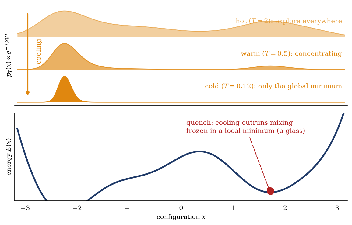
The central picture summarizes the argument (Figure 16.1): one rugged landscape, one family of Boltzmann distributions above it, and two possible fates below.

Figure 16.1: The lecture in one picture. Top: the Boltzmann distribution \(p_T \propto e^{-E(x)/T}\) over one rugged landscape at three temperatures — hot, the mass spreads over every basin (exploration); warm, it drains toward the deep wells; cold, only the global minimum survives. Bottom: the two fates of a cooled chain. Annealing — cooling slowly enough to stay near equilibrium at every temperature — tracks the concentrating distribution into the global minimum (the crystal); a quench — cooling faster than the chain can mix — strands it in a local minimum (a glass), exactly as in metallurgy.

16.2 The engine, part I: cooling concentrates

One landscape, a family of distributions. Fix the energy \(E(x)\) and let the temperature vary: Equation 1.2 becomes a one-parameter family

\[ p_T(x) \;=\; \frac{e^{-E(x)/T}}{Z_T}, \qquad Z_T = \sum_x e^{-E(x)/T}, \]

interpolating from the uniform distribution (\(T \to \infty\), where the exponent flattens completely) toward something increasingly selective as \(T\) falls. How selective, exactly? The question answers itself if we compare any state to the best one — and the comparison is the previous lecture’s central trick, because in a ratio the intractable \(Z_T\) cancels.

The concentration ratio. Let \(x^*\) be a global minimum of the energy, \(E^* = \min_x E(x)\), and let \(x\) be any state with \(E(x) > E^*\). Then

\[ \boxed{\; \frac{p_T(x)}{p_T(x^*)} \;=\; e^{-\left(E(x) - E^*\right)/T} \;\xrightarrow{\;T \to 0\;}\; 0 \;} \tag{16.1}\]

the \(T \to 0\) concentration

for every non-optimal state, however small its excess energy: any fixed gap \(E(x) - E^* > 0\) is eventually enormous compared to \(T\). All probability drains onto the global minima, and in the limit

\[ p_T \;\xrightarrow{\;T \to 0\;}\; \text{uniform on } \operatorname*{arg\,min}_x E(x) \]

— a single point mass if the minimum is unique, and the uniform distribution over all \(g\) ground states if it is \(g\)-fold degenerate (our spin-glass example below has \(g = 2\), the two global spin flips of one configuration). Temperature sets how sharply the Boltzmann distribution prefers low energy, and at \(T \to 0\) it prefers only the lowest — so a single sample from the zero-temperature limit is a certificate of global optimality. Optimization has become a sampling problem.

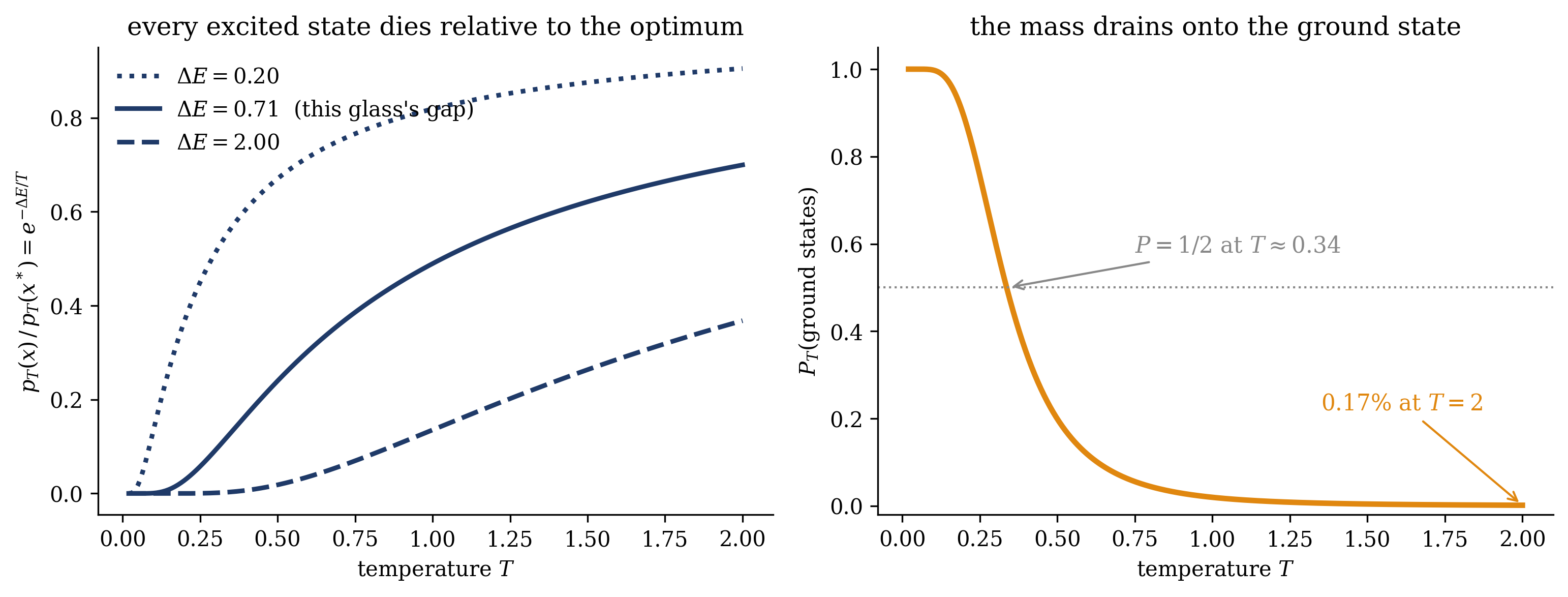
The free-energy reading. Week 1’s decomposition \(F = \langle E \rangle - TS\) says the same thing thermodynamically. At high temperature the entropy term dominates: the free energy is minimized by spreading — many states, all basins, exploration favored by the \(-TS\) term. As \(T\) falls, the entropic reward shrinks and the energy term takes over: the mass must commit to the lowest states, however few. Annealing is the walk this balance takes as \(T\) moves from one regime to the other, and the concentration Equation 16.1 is its destination. Figure 16.2 makes the statement quantitative on the very spin glass the worked example will anneal: sixteen spins, \(2^{16} = 65{,}536\) states enumerated exactly, and the total Boltzmann weight of the two ground states rising from \(0.17\%\) at \(T = 2\) (already a \(55\)-fold enhancement over the uniform \(2/65{,}536 \approx 0.003\%\)) through one half at \(T \approx 0.34\) to \(99\%\) by \(T \approx 0.12\).

Show code

N = 16

def make_glass(seed):
    rng = np.random.default_rng(seed)
    J = rng.normal(0, 1 / np.sqrt(N), (N, N))
    J = (J + J.T) / np.sqrt(2)
    np.fill_diagonal(J, 0.0)
    return J

J_a = make_glass(3)
S_all = np.array([[(c >> i & 1) * 2 - 1 for i in range(N)] for c in range(2**N)], dtype=float)
E_all = -0.5 * np.einsum("ci,ij,cj->c", S_all, J_a, S_all)
Estar_a = E_all.min()
is_ground = np.isclose(E_all, Estar_a)
gap = np.sort(np.unique(np.round(E_all - Estar_a, 9)))[1]

fig, (a1, a2) = plt.subplots(1, 2, figsize=(10.4, 4.0))

Ts = np.linspace(0.02, 2.0, 400)
for dE, ls in zip([0.2, gap, 2.0], [":", "-", "--"]):
    a1.plot(Ts, np.exp(-dE / Ts), color=NAVY, ls=ls, lw=2.2,
            label=rf"$\Delta E = {dE:.2f}$" + ("  (this glass's gap)" if np.isclose(dE, gap) else ""))
a1.set_xlabel(r"temperature $T$")
a1.set_ylabel(r"$p_T(x)\,/\,p_T(x^*) = e^{-\Delta E/T}$")
a1.set_title("every excited state dies relative to the optimum", fontsize=12)
a1.legend(frameon=False, fontsize=10, loc="upper left")

Pg = [np.exp(-(E_all - Estar_a) / T)[is_ground].sum() / np.exp(-(E_all - Estar_a) / T).sum()
      for T in Ts]
a2.plot(Ts, Pg, color=ORANGE, lw=2.6)
a2.axhline(0.5, color=GRAY, ls=":", lw=1)
a2.annotate(r"$P = 1/2$ at $T \approx 0.34$", xy=(0.34, 0.5), xytext=(0.75, 0.58),
            color=GRAY, fontsize=10.5,
            arrowprops=dict(arrowstyle="->", color=GRAY, lw=1))
a2.annotate(r"$0.17\%$ at $T = 2$", xy=(2.0, Pg[-1]), xytext=(1.35, 0.22),
            color=ORANGE, fontsize=10.5,
            arrowprops=dict(arrowstyle="->", color=ORANGE, lw=1))
a2.set_xlabel(r"temperature $T$")
a2.set_ylabel(r"$P_T(\mathrm{ground\ states})$")
a2.set_title("the mass drains onto the ground state", fontsize=12)
a2.set_ylim(-0.02, 1.05)
fig.tight_layout()
plt.show()

Figure 16.2: Concentration, exactly, on the spin glass of the worked example (\(N = 16\) spins, couplings \(J_{ij} \sim \mathcal{N}(0, 1/N)\), all \(65{,}536\) states enumerated). Left: the boxed ratio Equation 16.1 for three energy gaps — the middle curve uses this instance’s actual first excitation gap \(\Delta E = 0.71\). Every non-optimal state’s relative weight dies as \(T \to 0\); bigger gaps die sooner. Right: the total Boltzmann probability of the two degenerate ground states against temperature. At \(T = 2\) they carry \(0.17\%\) of the mass; the curve crosses \(1/2\) at \(T \approx 0.34\) and reaches \(99\%\) by \(T \approx 0.12\) — a sample from the cold distribution is, with overwhelming probability, the exact optimum. The entire remaining question is whether a chain can *follow* this curve down.

16.3 The engine, part II: the schedule and the quench

Why you cannot simply set \(T = 0\). Put \(T = 0\) into the previous lecture’s acceptance rule Equation 15.2: every uphill acceptance \(e^{-\Delta E/T}\) vanishes, and the chain accepts only moves that lower the energy — greedy descent. Such a chain stops, permanently, at the first configuration from which every move goes uphill: a local minimum, and almost never the global one. Our sixteen-spin glass has \(28\) of these single-flip-stable states, and greedy descent from a random start reaches the true ground state in only \(29\%\) of runs — the other \(71\%\) end in one of the \(26\) impostors. Sampling at \(T = 0\) is precisely the trapping we set out to avoid; the zero-temperature limit is a destination to approach, never an operating point. So the chain must start hot, where barriers are crossable, and cool: run Metropolis with a time-dependent temperature \(T(t)\), decreasing from exploration to commitment. Everything now hangs on how fast.

The constraint is the previous lecture’s mixing time. The concentration argument of Section 16.2 is a statement about equilibrium at each temperature; the chain inherits its benefits only if it actually equilibrates as it cools. Equilibration at temperature \(T\) costs the mixing time \(\tau(T)\) — and \(\tau(T)\) grows as \(T\) falls, because barrier crossings are exponentially suppressed: a barrier of height \(\Delta B\) takes of order \(e^{\Delta B/T}\) attempts (the Arrhenius law W9 will derive from Langevin dynamics; today it is the previous lecture’s uphill-acceptance rule read as a waiting time). Cooling therefore races against a clock that runs slower the colder it gets, and the race has exactly two outcomes. Cool within the clock, and the chain stays near \(p_{T(t)}\) at every moment and is carried onto the ground state. Outrun the clock, and the chain falls out of equilibrium and freezes wherever it stands — the quench, and the frozen result is a glass in exactly the metallurgist’s sense: a configuration held in place not because it is good but because the moves that would improve it have become too expensive to afford.

The quench, priced. “Frozen wherever it stands” can be made quantitative with Week 1’s free-energy decomposition and the previous lecture’s adjoint kernel (Welling, Lu, and Holdijk 2026, ch. 10 on stochastic thermodynamics). Define the nonequilibrium free energy of whatever distribution \(\rho\) the chain currently carries, \(F[\rho] = \langle E \rangle_\rho - T\, S[\rho]\) — Week 1’s decomposition, now evaluated off equilibrium. Two lines relate it to the equilibrium value \(F_T = -T \log Z_T\): since \(-\log p_T(x) = E(x)/T + \log Z_T\),

\[ F[\rho] - F_T \;=\; \langle E \rangle_\rho + T \langle \log \rho \rangle_\rho + T \log Z_T \;=\; T\, \big\langle \log \rho - \log p_T \big\rangle_\rho \;=\; T\; D_\mathrm{KL}\big(\rho \,\|\, p_T\big) \;\geq\; 0 . \tag{16.2}\]

excess free energy = KL to equilibrium

Every distribution sits above equilibrium by an excess free energy, and the excess is its Kullback–Leibler divergence to the Boltzmann distribution, priced in units of \(T\). Relaxation drains this excess monotonically, and the proof needs only the machinery from the previous lecture. Write the joint law of one chain step in two ways: seeded at \(\rho\), it is \(q(x, x') = \rho(x)\, W(x \to x')\); seeded at equilibrium, \(r(x, x') = p_T(x)\, W(x \to x')\). In the ratio \(q/r\) the kernels cancel, so \(D_\mathrm{KL}(q \| r) = D_\mathrm{KL}(\rho \| p_T)\). Now decompose the same divergence by conditioning on the endpoint instead: the marginals are \(\rho W\) and \(p_T W = p_T\), the equilibrium conditional \(r(x \mid x')\) is the previous lecture’s adjoint kernel (Equation 15.3, making its second appearance), and the chain rule for KL gives

\[ D_\mathrm{KL}(\rho \| p_T) \;=\; D_\mathrm{KL}\big(\rho W \,\|\, p_T\big) + \underbrace{\big\langle D_\mathrm{KL}\big( q(\cdot \mid x') \,\|\, r(\cdot \mid x') \big) \big\rangle_{\rho W}}_{\geq\, 0} \;\;\Longrightarrow\;\; D_\mathrm{KL}\big(\rho W \,\|\, p_T\big) \;\leq\; D_\mathrm{KL}\big(\rho \,\|\, p_T\big) . \]

Each sweep of the chain lowers the excess free energy, with equality only at equilibrium — a discrete H-theorem, and the information theorist’s data-processing inequality in physical units. An anneal is now a sequence of these drains against moving targets: at each stage the chain sheds divergence toward \(p_{T_k}\), then the cooling step sharpens the target and re-prices what remains. End the schedule before the drain completes and the residual \(D_\mathrm{KL}(\rho_\text{end} \| p_{T_\text{end}})\) is frozen in: by Equation 16.2 it is exactly the glass’s excess free energy over the crystal, and the quench trace of Figure 16.4 flattening above the dotted ground-state line is this residual, seen in its energy component. Week 9 takes this monotone descent to continuous time, where it becomes the H-theorem of the Fokker–Planck equation, and Week 11 refines the accounting to single trajectories, where the drained divergence acquires the name entropy production and the frozen residual returns as the dissipated work of a finite-time protocol.

The guaranteed schedule — and its price. Geman and Geman (1984) made “slow enough” precise:

\[ T(t) \;\geq\; \frac{c}{\log(1 + t)} \quad \Longrightarrow \quad \text{convergence to the global minima, almost surely} \tag{16.3}\]

logarithmic cooling (guaranteed)

where the constant \(c\) must be at least the depth of the deepest barrier around a non-global minimum — that sharp, necessary-and-sufficient value is Hajek (1988)’s; Geman and Geman (1984)’s original proof guaranteed convergence for a larger \(c \sim N\Delta\) (sites times energy range) — and the schedule must additionally send \(T(t) \to 0\), since a constant temperature satisfies the inequality as written yet converges to nothing. The theorem is genuine, and its fine print undoes it in practice: inverting the schedule, reaching temperature \(T\) takes \(t \sim e^{c/T}\) steps — the same exponential as the barrier crossings the schedule must wait for. A guarantee that costs the age of the universe on a modest instance is a guarantee in name only; nobody anneals logarithmically. What practice uses instead is

\[ T_{k+1} = \alpha\, T_k, \qquad \alpha \in (0.8,\, 0.99) \tag{16.4}\]

geometric cooling (practical)

— a fixed multiplicative decay per stage, fast, tunable, and backed by no theorem at all. The pairing is a shape this course keeps meeting: the schedule with the proof is unusable, and the schedule in use is unproven. Simulated annealing is a powerful heuristic — it beats greedy descent wherever barriers matter — but it is not a guaranteed global optimizer at any practical cooling rate, and results obtained with it should be reported with that in mind. (One notational flag while the symbols are fresh: \(\alpha\) here is the cooling factor, not Week 2’s storage load; and \(T(t)\) is now a program, not a parameter — \(\beta = 1/T\) climbs as the schedule runs.)

Trap

\(T = 0\) is a limit, not a temperature — and the guarantee is not a license. There are two traps. ① Sampling at \(T = 0\) is greedy descent: on the example glass it fails \(71\%\) of the time. The optimizer is the approach — the schedule — never the endpoint; a chain parked at any fixed low \(T\) simply inherits the previous lecture’s exponential mixing time. ② The logarithmic guarantee Equation 16.3 requires \(t \sim e^{c/T}\) steps with \(c\) set by the deepest barrier — real and unusable. Every practical anneal is a heuristic, and a reported “optimum” from geometric cooling is a best-found, not a certificate.

Take-home 2

You cannot sample at \(T = 0\) (greedy descent, trapped); you must cool, and no faster than the chain mixes at each temperature — a clock that itself slows as \(e^{\Delta B/T}\). Logarithmic cooling \(T \geq c/\log(1+t)\) guarantees the global minimum (Geman and Geman (1984)) at an exponential, unusable price; geometric cooling \(T_{k+1} = \alpha T_k\) is the practical, unguaranteed compromise. Cooling faster than mixing is a quench: frozen in a glass, exactly where mixing is worst — through \(T_c\) and in rugged landscapes.

16.4 The bridge: the learning rate is a temperature

High temperature buys exploration — the chain accepts bad moves and visits basins it would never enter greedily; low temperature buys exploitation — it refines what it has. Annealing is the disciplined handover from one to the other, and stated this way the idea is not about spins at all: every stochastic optimizer manages the same trade, and every practitioner of deep learning already schedules a knob that does exactly this. The correspondence is literal.

Consider noisy gradient descent on a loss \(L(\theta)\), with the noise injected deliberately:

\[ \theta_{t+1} \;=\; \theta_t \;-\; \eta\, \nabla L(\theta_t) \;+\; \sqrt{2\,\eta\, T}\; \xi_t, \qquad \xi_t \sim \mathcal{N}(0, \mathbb{1}), \]

a downhill step of size \(\eta\) plus a Gaussian kick. This is the discretization of Langevin dynamics, and Week 9’s engine (the Fokker–Planck equation) will prove what today we only state: its stationary distribution is \(\propto e^{-L(\theta)/T}\) — a Boltzmann distribution over the loss landscape, with the loss as energy. Run at \(T = 1\) with mini-batch gradients, this is precisely stochastic gradient Langevin dynamics (Welling and Teh 2011), a sampler for Bayesian posteriors built from an optimizer; the tutorial compares its samples to an exact posterior. Now delete the injected noise and run plain SGD. The randomness does not vanish — the mini-batch gradient is itself a noisy estimate, with a covariance set by the data and the batch size, independent of \(\eta\). Carried through the same dynamics, drift scales as \(\eta\) while the noise’s variance scales as \(\eta^2\), and the ratio that plays the role of temperature comes out proportional to the step size:

\[ \boxed{\; T_\text{eff} \;\propto\; \eta \qquad \Longrightarrow \qquad \text{a learning-rate schedule is a cooling schedule} \;} \tag{16.5}\]

temperature ↔︎ learning rate

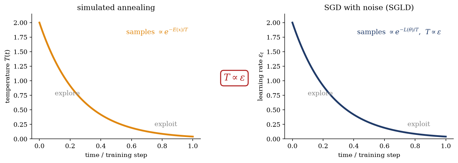
Decaying \(\eta_t\) over training is annealing on the loss (Figure 16.3): the large early steps are the hot phase, roaming among basins; the small late steps are the cold phase, committing to one and refining it. The warm-up schedules, step decays, and cosine schedules of deep-learning practice are cooling schedules, tuned by exactly the trade this lecture formalized — and the quench has a training-room name too: drop the learning rate too early and the run freezes into whichever basin it happened to occupy, the optimizer’s glass. One caveat: for SGLD the Boltzmann stationary distribution is a theorem (in the decreasing-step limit; at a fixed step there is an \(\mathcal{O}(\eta)\) discretization bias); for plain SGD, \(T_\text{eff} \propto \eta\) is today a scaling argument, and turning it into a precise statement — what exactly SGD’s mini-batch noise does, when the Boltzmann form holds, and what it says about flat minima and generalization — is the entire business of Week 9. (Two script-only pointers for the curious: parallel tempering, the modern cure for glassy annealing — run replicas at a ladder of temperatures and swap them, so cold chains borrow the hot chains’ mobility; and annealed importance sampling, Week 11, where a cooling schedule is used not to optimize but to estimate \(Z\) itself.)

Figure 16.3: The same knob, two rooms. Left: simulated annealing schedules a temperature \(T(t)\) downward; the chain samples \(\propto e^{-E(x)/T}\) and passes from exploration to exploitation. Right: SGD with a decaying learning rate \(\eta_t\) does the same on a loss landscape — Langevin dynamics samples \(\propto e^{-L(\theta)/T}\) with \(T \propto \eta\), so the learning-rate schedule is a cooling schedule. Week 9 derives the correspondence; the tutorial runs it.

Take-home 3

Temperature trades exploration for exploitation, and in learning that knob is the learning rate: Langevin dynamics with step \(\eta\) and temperature \(T\) has stationary distribution \(\propto e^{-L/T}\) (SGLD, Welling and Teh (2011)), and plain SGD’s mini-batch noise gives \(T_\text{eff} \propto \eta\). Decaying the learning rate is cooling; SGD with a decaying step is simulated annealing on the loss; and dropping the rate too early is a quench. Week 9 turns the scaling argument into a theorem.

16.5 Example: anneal versus quench, on sixteen spins

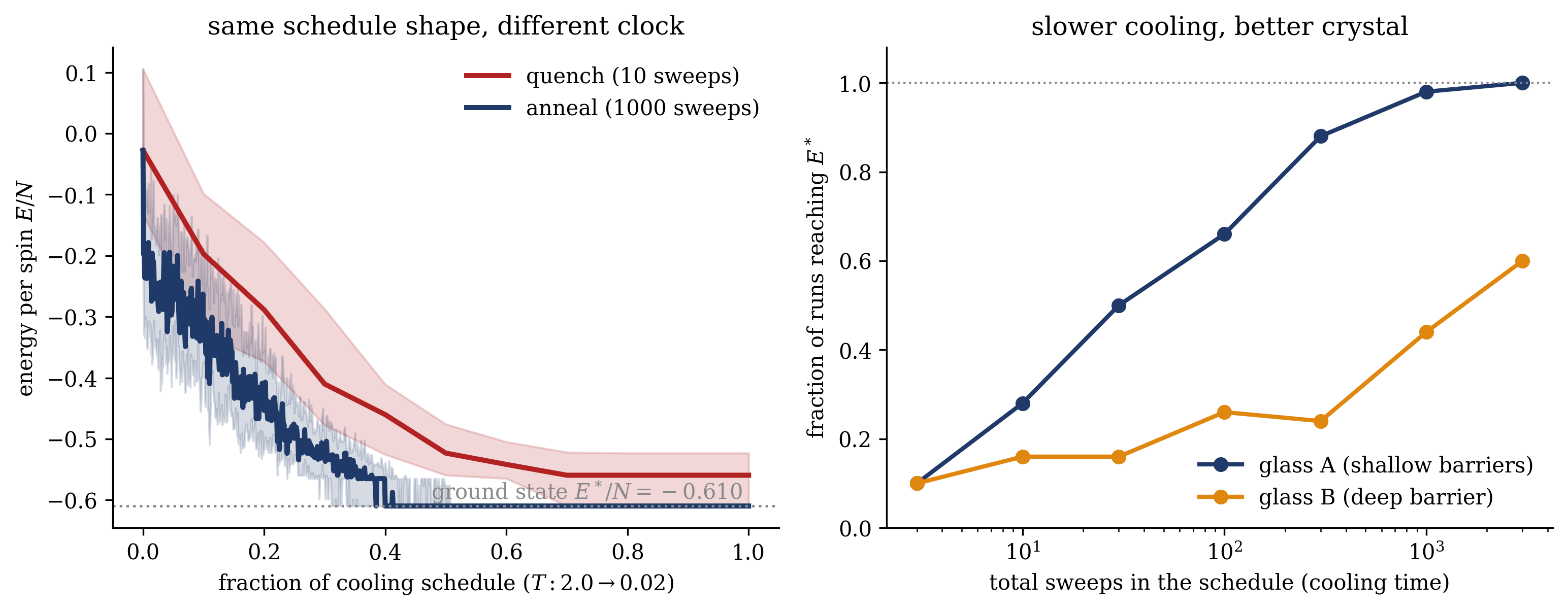
A single enumerable instance illustrates the claims. Take the spin glass of Figure 16.2 — \(N = 16\), \(J_{ij} \sim \mathcal{N}(0, 1/N)\), all \(65{,}536\) states enumerated, ground-state energy \(E^*/N = -0.610\) (doubly degenerate, the global flip) and \(28\) local minima — and anneal it with Metropolis under geometric cooling from \(T = 2.0\) to \(0.02\), giving the schedule different total durations. Every run uses the same schedule shape; only the clock changes. For contrast, a second instance from the same ensemble (“glass B”, \(E^*/N = -0.599\)) whose dominant barrier happens to be deeper. Fifty independent runs per point; Figure 16.4 shows the traces and the verdict, and the fractions of runs that end in the true ground state read:

total sweeps	3	10	30	100	300	1000	3000	greedy (\(T=0\))
glass A	\(0.10\)	\(0.28\)	\(0.50\)	\(0.66\)	\(0.88\)	\(0.98\)	\(1.00\)	\(0.29\)
glass B	\(0.10\)	\(0.16\)	\(0.16\)	\(0.26\)	\(0.24\)	\(0.44\)	\(0.60\)	\(0.20\)

Slower cooling monotonically improves the crystal: on glass A the success rate climbs from \(10\%\) for a three-sweep quench to certainty at three thousand sweeps — the anneal–quench crossover of Section 16.3 as a measured curve. The greedy column calibrates both ends: pure descent manages \(29\%\), roughly a third of a patient anneal’s success rate, yet still beats the fastest quenches — which end their schedule before they have finished descending at all. And glass B makes Hajek’s constant \(c\) concrete: same size, same ensemble, one deeper barrier, and every entry drops — at three thousand sweeps, where glass A is solved, glass B still fails four times in ten. The schedule a landscape demands is set by its deepest barrier, exponentially; no single cooling rate is “slow enough” in general, which is why Equation 16.3’s guarantee had to be logarithmic and why annealing remains a heuristic. In the traces (left panel), the story is visible directly: the quench’s median energy flattens at \(-0.56\) per spin, an excited glass, while the anneal’s median lands on the dotted ground-state line at \(-0.610\).

Show code

def anneal_ensemble(J, sweeps, runs, T0=2.0, T1=0.02, seed=0, trace=False):
    """`runs` independent Metropolis chains, cooled geometrically from T0 to T1."""
    rng = np.random.default_rng(seed)
    s = rng.choice([-1.0, 1.0], (runs, N))
    E = -0.5 * np.einsum("ri,ij,rj->r", s, J, s)
    alpha = (T1 / T0) ** (1 / max(sweeps - 1, 1))
    T = T0
    traces = [E.copy()]
    for k in range(sweeps):
        for _ in range(N):                       # one sweep = N attempted flips
            i = rng.integers(N, size=runs)
            dE = 2 * s[np.arange(runs), i] * np.einsum("rj,rj->r", J[i], s)
            acc = (dE <= 0) | (rng.random(runs) < np.exp(-np.clip(dE, 0, None) / T))
            s[np.arange(runs), i] = np.where(acc, -s[np.arange(runs), i], s[np.arange(runs), i])
            E = np.where(acc, E + dE, E)
        T *= alpha
        if trace:
            traces.append(E.copy())
    return (np.array(traces), E) if trace else E

J_b = make_glass(4)   # ground state via the S_all enumeration of the previous cell
Estar_b = (-0.5 * np.einsum("ci,ij,cj->c", S_all, J_b, S_all)).min()

fig, (a1, a2) = plt.subplots(1, 2, figsize=(10.4, 4.1))

tr_slow, _ = anneal_ensemble(J_a, 1000, 50, seed=1, trace=True)
tr_fast, _ = anneal_ensemble(J_a, 10, 50, seed=1, trace=True)
for tr, sw, col, lab in [(tr_fast, 10, RED, "quench (10 sweeps)"),
                         (tr_slow, 1000, NAVY, "anneal (1000 sweeps)")]:
    x = np.linspace(0, 1, sw + 1)
    lo, mid, hi = np.percentile(tr / N, [25, 50, 75], axis=1)
    a1.fill_between(x, lo, hi, color=col, alpha=0.18)
    a1.plot(x, mid, color=col, lw=2.4, label=lab)
a1.axhline(Estar_a / N, color=GRAY, ls=":", lw=1.2)
a1.text(0.99, Estar_a / N + 0.012, r"ground state $E^*/N = -0.610$",
        color=GRAY, fontsize=10, ha="right")
a1.set_xlabel(r"fraction of cooling schedule ($T: 2.0 \to 0.02$)")
a1.set_ylabel(r"energy per spin $E/N$")
a1.set_title("same schedule shape, different clock", fontsize=12)
a1.legend(frameon=False, fontsize=10, loc="upper right")

budgets = [3, 10, 30, 100, 300, 1000, 3000]
for J, Estar, col, lab in [(J_a, Estar_a, NAVY, "glass A (shallow barriers)"),
                           (J_b, Estar_b, ORANGE, "glass B (deep barrier)")]:
    fr = [np.isclose(anneal_ensemble(J, sw, 50, seed=7), Estar).mean() for sw in budgets]
    a2.semilogx(budgets, fr, "o-", color=col, lw=2, ms=6, label=lab)
a2.axhline(1.0, color=GRAY, ls=":", lw=1)
a2.set_xlabel("total sweeps in the schedule (cooling time)")
a2.set_ylabel(r"fraction of runs reaching $E^*$")
a2.set_title("slower cooling, better crystal", fontsize=12)
a2.set_ylim(0, 1.08)
a2.legend(frameon=False, fontsize=10, loc="lower right")
fig.tight_layout()
plt.show()

Figure 16.4: Anneal versus quench on glass A (\(N = 16\); exact \(E^*/N = -0.610\) from enumeration; geometric cooling \(T: 2.0 \to 0.02\)). Left: median energy per spin with interquartile band over \(50\) runs, plotted against the *fraction* of the schedule — the quench (red, \(10\) sweeps total) and the anneal (navy, \(1000\) sweeps) follow identical schedule shapes with different clocks. The quench freezes at \(-0.56\) per spin, an excited local minimum; the anneal tracks equilibrium and lands on the ground state. Right: the fraction of \(50\) runs ending in the true ground state against the total schedule length, for glass A and for a second instance with a deeper dominant barrier. Slower cooling always helps; how slow is *enough* is set by the deepest barrier — glass B still fails \(40\%\) of the time at a budget that solves glass A completely. The metallurgical claim — slow cooling makes crystals, fast cooling makes glasses — is here a measured curve.

Anneal to optimize: cool slowly enough to stay in equilibrium — a quench traps you in a glass, and a learning-rate schedule is a cooling schedule.

The tutorial (16–18, Ph12 106) is derivation-led. Two problems. First, simulated annealing on the travelling salesman problem — you will watch a tour untangle as the temperature drops, and choose the schedule yourselves; The warm-up card already gave you Kirkpatrick, Gelatt, and Vecchi (1983), where that exact problem earned the method its name. Second, stochastic gradient Langevin dynamics against an exact Bayesian posterior — take Equation 16.5’s claim into the room and test it on a model small enough to integrate by hand. The tutorial requires no devices.

16.6 Outlook: from cooling to training

Week 8 closes with the sampling road fully open and its first two uses in hand. The previous lecture established that the Boltzmann distribution can be sampled without its normalizer, at the price of mixing; today made the sampler’s one knob into an instrument, and the price reappeared as the quench — every claim of this lecture was ultimately a claim about mixing under a deadline. That the resulting algorithm was invented by a spin-glass physicist is not incidental: the rugged landscapes where annealing is both necessary and hard are the same ones Weeks 2 and 6 mapped, and the metallurgical vocabulary — crystal, glass, quench — has been the course’s vocabulary for memory and optimization since Figure 3.1.

Week 9 is the module’s destination, and today’s bridge is its on-ramp. The claim \(T_\text{eff} \propto \eta\) was offered as a scaling argument; next week supplies the machinery — Langevin dynamics as the continuum limit of noisy descent, the Fokker–Planck equation as its law of motion, and the Boltzmann distribution over the loss as its stationary state — and with it the striking consequences: why SGD’s noise selects flat minima, what that has to do with generalization, and why the training hyperparameters everyone tunes are thermodynamic variables under other names. Training is sampling; this week built the sampler, and next week reads the training loop as one.

The longer thread runs to the course’s title. Cooling as a computational principle does not end with optimization: Week 11 anneals to estimate the very \(Z\) this module dodges (annealed importance sampling — a bridge of intermediate temperatures between a tractable distribution and the target), and Week 12’s diffusion models are, at heart, an annealing schedule run as a generative process — noise added along a schedule and removed along the reverse one, with a learned denoiser standing where the Metropolis rule stands today. The annealing framework, introduced in a 1983 Science paper, remains active through the final lecture.