21Fluctuation theorems: buying \(\log Z\) with irreversible work
Recommended reading
Core (~1 h).Jarzynski (1997) — four pages, and the warm-up reading for the next lecture: an equality where 170 years of thermodynamics had only the inequality \(\langle W\rangle \ge \Delta F\). Drive a system from equilibrium at \(A\) to \(B\) at any finite speed, measure the work trajectory by trajectory, and \(\langle e^{-\beta W}\rangle = e^{-\beta \Delta F}\) exactly. The paper derives it from Hamiltonian dynamics; today we take the discrete Markov route instead — read it for the statement and the estimator reading. Alongside it, Crooks (1999) — the sharper parent: not one average but the whole forward and reverse distributions of work, locked together and crossing at \(\Delta F\). Our engine follows its detailed-balance logic.
Optional background.Jarzynski (2011) — the retrospective review, the cleanest survey of what the work relations do and do not say; Liphardt et al. (2002) and Collin et al. (2005) — the theorems verified by pulling single RNA molecules, equilibrium folding free energies read off irreversible pulls (the experimental hook); Sohl-Dickstein et al. (2015) — read the title and introduction only: the founding diffusion paper, built on exactly this literature; Neal (2001) — the next lecture’s subject, the estimator engineered, skim §1 if curious.
Prerequisite reminder. The canonical distribution \(p = e^{-\beta E}/Z\) and \(F = -T\log Z\) (Week 1); detailed balance and Markov kernels with Boltzmann stationary laws (Chapter 15, Equation 15.1); the forward/reverse process picture of Chapter 20. New content: driving protocols and trajectory work, the Crooks and Jarzynski relations, the abstract fluctuation-theorem identity from which both fall out, dissipation as a forward/reverse KL divergence, and free-energy estimation from nonequilibrium trajectories.
21.1 The remaining problem
Week 10 completed what the course began in Week 3. Its first lecture removed the partition function from training — the score \(\nabla_x \log p = -\nabla_x E\) is blind to \(Z\) (Equation 19.1) — and its second removed it from generation, with Anderson’s reverse-time SDE (Equation 20.2) turning a fixed corruption process into an exact generator. Between the two, every obstruction the course had fought was dissolved or bypassed — except one, which has been outstanding since Module 3.
Recall the escape from \(Z\) that opened Week 8 (Chapter 15): to sample\(p \propto e^{-\beta E}\) you never need \(Z\), because it cancels in every ratio \(p(x')/p(x) = e^{-\beta \Delta E}\). That cancellation is exactly why Markov chain Monte Carlo works — and exactly why it can never hand you \(Z\) itself. A sampler reports averages; it does not report the normalizer, and so it cannot compare two models by likelihood, cannot report a free energy, cannot tell you how probable a configuration is, only how probable it is relative to another. Module 3 noted this limitation and deferred the resolution.
The problem is tractable once it is restated. We almost never want \(Z\) alone; we want comparisons — and a comparison of two partition functions is a free-energy difference,
\[
\Delta F \;=\; F_B - F_A \;=\; -T\,\log\frac{Z_B}{Z_A},
\tag{21.1}\]
free energy as a ratio of partition functions
a ratio of the two forbidden numbers. And here is the lever: if \(A\) is a tractable reference — independent spins, a Gaussian, anything whose \(Z_A\) is known in closed form — then an estimator of \(\Delta F\)is an estimator of \(\log Z_B\). The absolute value of \(\log Z_B\) is one subtraction from a ratio that can be estimated.
What nonequilibrium statistical mechanics discovered, in a burst between 1997 and 1999, is that this ratio is cheap to estimate. Jarzynski (1997) proved that if you drive a system from equilibrium at \(A\) to the control setting of \(B\) in finite time — however fast, however far from equilibrium — and record the work \(W\) expended along each stochastic trajectory, then
an exact equality at any driving speed, where thermodynamics since Clausius had offered only \(\langle W\rangle \ge \Delta F\). Two years later Crooks (1999) found the sharper statement from which Jarzynski’s falls out in one line: the entire distributions of work in the forward and time-reversed protocols are locked together, and cross at exactly \(W = \Delta F\). These are exact identities, not near-equilibrium approximations, and they turn driven, irreversible trajectories into an unbiased estimator of \(\log Z\) — the quantity that has been inaccessible throughout the course. Module 3 sampled without \(Z\); this week estimates it.
The identities were not idle theory for long. Liphardt et al. (2002) and then Collin et al. (2005) pulled single RNA hairpins open with optical tweezers — a strongly irreversible operation — and recovered the molecules’ equilibrium folding free energies from the work histograms, reading \(\Delta F\) off the point where the forward and reverse distributions cross. And downstream, the same machinery became an algorithm: Neal (2001) turned Jarzynski’s identity into annealed importance sampling (the next lecture), and Sohl-Dickstein et al. (2015) built the first diffusion model on this literature — the paper is titled Deep Unsupervised Learning using Nonequilibrium Thermodynamics. A familiar historical pattern: a physics result waiting decades for machine learning to need it (Onsager 1936 for TAP, Bethe 1935 for belief propagation, Anderson 1982 for the reverse-time SDE, and now Jarzynski and Crooks for the diffusion training bound).
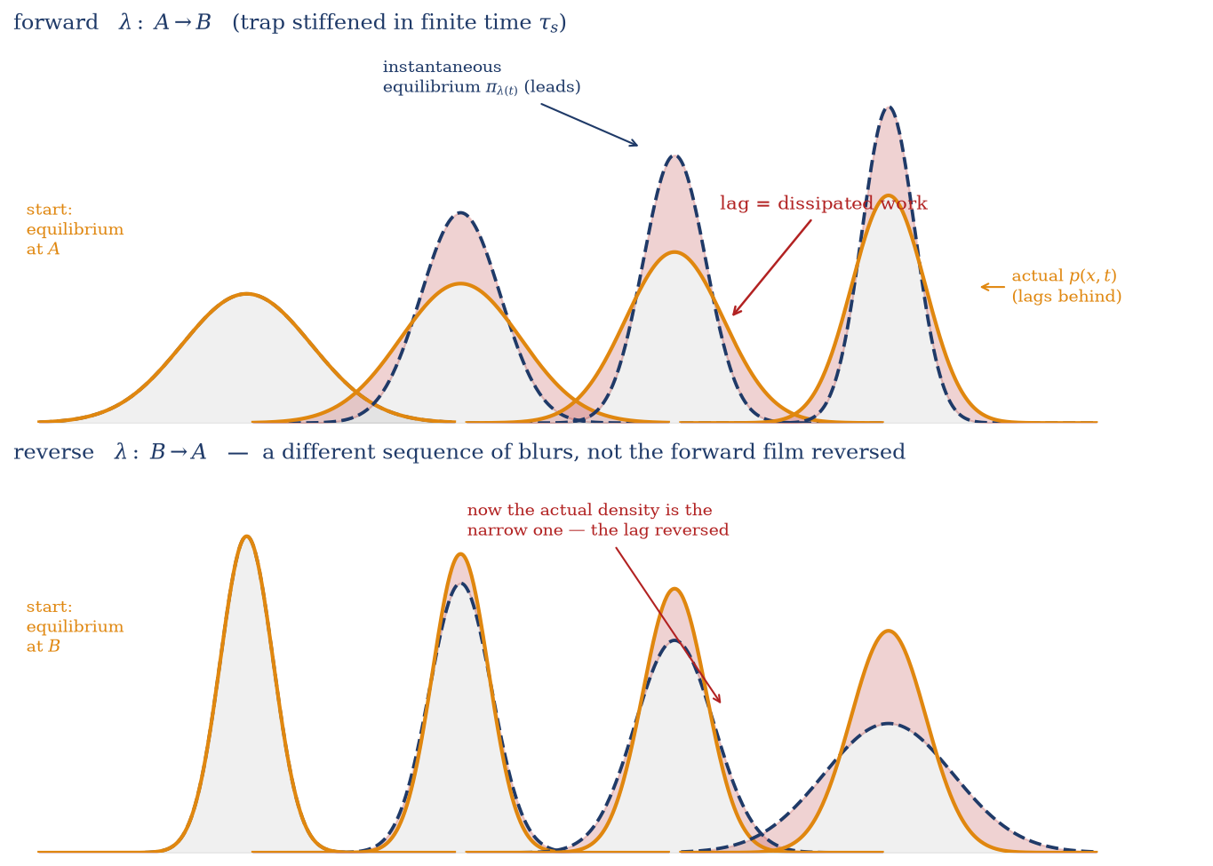
Figure 21.1 summarizes the setup. A control parameter \(\lambda(t)\) is driven from \(A\) to \(B\) in finite time — a trap stiffened, a piston pushed, a field ramped. Drive it slowly and the system stays in the instantaneous equilibrium \(\pi_{\lambda(t)}\) throughout; drive it fast and the actual distribution \(p(x,t)\)lags behind, and the shaded gap between them is paid as dissipated work. The reverse protocol, run from equilibrium at \(B\) back to \(A\), generates a different sequence of lagging distributions — it is not the forward film played backwards. Crooks’ theorem is the precise statement that the dissipated work measures exactly how different those two films are.
Figure 21.1: The central picture. A control parameter \(\lambda(t)\) is driven in finite time, here a harmonic trap \(E_\lambda(x) = \tfrac12 k(\lambda)\,x^2\) stiffened from \(A\) to \(B\) (top) and softened from \(B\) back to \(A\) (bottom); the curves are the exact time-marginals of the overdamped dynamics. Top: the instantaneous equilibrium \(\pi_{\lambda(t)}\) (navy dashed) contracts as the trap stiffens, but the actual density \(p(x,t)\) (orange) lags behind, still too wide — the red gap is the lag that the dissipated work pays for (it bounds the dissipation, Equation 21.5). Bottom: run in reverse the lag flips sign — the actual density is now the narrow one, still remembering the stiff trap it started in. The forward and reverse sequences of blurs are genuinely different, and (Crooks) their difference is exactly what the second law charges for finite-time driving. This is Week 10’s filmstrip with a price tag.
Classical thermodynamics answers the finite-time question with a bound and two useless limits. The bound is \(\langle W\rangle \ge \Delta F\), with equality only in the quasistatic limit. So to extract \(\Delta F\) classically you have two options, and both fail. Drive infinitely slowly (thermodynamic integration): exact, but it costs infinite time. Or switch instantly and reweight (free-energy perturbation, Zwanzig (1954)): fast, but its variance is hopeless. The question: what does a finite-time, irreversible protocol know about \(\Delta F\)?\(\Delta F\) is fully determined by the work fluctuations, provided one averages the right function.
Take-home 1
Free-energy differences are ratios of partition functions, \(\Delta F = -T\log(Z_B/Z_A)\) (Equation 21.1); with a tractable reference \(A\), estimating \(\Delta F\) estimates \(\log Z_B\) — the number MCMC (Module 3) could never deliver, because \(Z\) cancels in the ratios sampling relies on. The fluctuation theorems extract that number from finite-time, irreversible driving: the information the second law’s inequality discards survives in the fluctuations of the work.
21.2 The discrete protocol: work and heat on the course’s own machinery
To track a driven system exactly we discretize the protocol into two elementary moves and account for each on the vocabulary Week 8 already built. Introduce an interpolating family of energies
\[
E_k(x) = E(x;\lambda_k), \qquad k = 0, 1, \dots, N, \qquad E_0 = E_A,\; E_N = E_B,
\]
with the corresponding equilibrium distributions \(p_k(x) = e^{-\beta E_k(x)}/Z_k\). This is the ladder annealed importance sampling will engineer in the next lecture and the ladder diffusion makes continuous in Week 12; for now it is just a fine subdivision of the drive from \(A\) to \(B\). A single step of the protocol is the composition of two moves:
① Work step. Switch the energy \(E_{k-1} \to E_k\) at frozen configuration \(x\). The system does not move, so no heat is exchanged; the change in energy is charged to the driver as work, \[
w_k = E_k(x) - E_{k-1}(x).
\]
② Heat step. Move the configuration by a Markov kernel \(T_k(x \to x')\) that is detailed-balanced with respect to \(p_k\) — Week 8’s boxed condition (Equation 15.1), \(T_k(x\to x')\,p_k(x) = T_k(x'\to x)\,p_k(x')\), applied at fixed \(\lambda_k\). The energy changes because \(x\) moves, and that change is heat exchanged with the bath; no work is done.
A forward trajectory draws \(x_0 \sim p_0\) from equilibrium at \(A\) and then alternates: work step to \(\lambda_1\), heat step at \(\lambda_1\) producing \(x_1\), work step to \(\lambda_2\), heat step producing \(x_2\), and so on to \(x_N\). The total work along the trajectory is the sum of the work steps only,
each term evaluated at the configuration before the heat step that follows. This is the trajectory analogue of the first law: the energy change from moving \(\lambda\) at frozen \(x\) is work, the energy change from moving \(x\) at fixed \(\lambda\) is heat, and \(W\) collects the former. Conflating \(W\) with the naive endpoint difference \(E_B(x_N) - E_A(x_0)\) — which also folds in all the heat — breaks every identity below; the work is the driver’s ledger, not the system’s energy budget.
The reverse process starts from equilibrium at \(B\), \(x_N \sim p_N\), and runs the protocol backwards, \(\lambda_N \to \lambda_0\), applying the same kernels in reversed order. One point matters now because it is persistently misread: only the initial state of each process need be in equilibrium. The forward process starts from \(p_A\) and the reverse from \(p_B\); nothing is assumed to equilibrate along the way, and nothing need reach equilibrium at the far end. The theorems hold regardless of how far from equilibrium the driving pushes the system. Every object on the board so far is Week 8’s — Boltzmann weights and detailed-balanced kernels — and the only new element is the bookkeeping of a moving \(\lambda\). With that in place the ratio of the forward and reverse path probabilities is a three-line computation.
21.3 The engine: the path ratio, Crooks, Jarzynski
Compare the probability of a forward trajectory with the probability of the same configurations visited in reverse order under the reverse protocol.
Step 1 — path probabilities. The forward trajectory \(x = (x_0, x_1, \dots, x_N)\) has probability \[
P_F[x] \;=\; p_0(x_0)\,\prod_{k=1}^{N} T_k(x_{k-1} \to x_k),
\] the equilibrium start times the product of the heat-step kernels. The reversed trajectory \(\tilde x = (x_N, \dots, x_0)\) under the reverse protocol has probability \[
P_R[\tilde x] \;=\; p_N(x_N)\,\prod_{k=1}^{N} T_k(x_k \to x_{k-1}),
\] with the same kernels traversed in the opposite direction.
Step 2 — detailed balance flips each kernel. The one identity we use, once per step, is Equation 15.1: \[
T_k(x_k \to x_{k-1}) \;=\; T_k(x_{k-1} \to x_k)\,\frac{p_k(x_{k-1})}{p_k(x_k)}.
\] Every forward kernel factor cancels against its reverse partner; what survives is a ratio of Boltzmann weights.
Step 3 — the telescoping. Substituting and cancelling the kernels, \[
\frac{P_R[\tilde x]}{P_F[x]}
\;=\; \frac{p_N(x_N)}{p_0(x_0)} \prod_{k=1}^{N} \frac{p_k(x_{k-1})}{p_k(x_k)}
\;=\; \prod_{k=1}^{N} \frac{p_k(x_{k-1})}{p_{k-1}(x_{k-1})}
\;=\; \prod_{k=1}^{N} \frac{Z_{k-1}}{Z_k}\,e^{-\beta[E_k(x_{k-1}) - E_{k-1}(x_{k-1})]}.
\] The middle equality is the telescoping: the boundary factors \(p_N(x_N)\) and \(1/p_0(x_0)\) are absorbed as the \(k=N\) and \(k=1\) ends of the shifted product \(\prod_k p_k(x_{k-1})/p_{k-1}(x_{k-1})\). Now the two surviving pieces are exactly the quantities we named. The product of partition-function ratios telescopes to \(Z_0/Z_N = Z_A/Z_B = e^{\beta \Delta F}\) (Equation 21.1), and the exponent is precisely the total work (Equation 21.2). Both collapse:
How much less probable the reversed movie is than the forward one is set by exactly the work you wasted: dissipation is time-reversal asymmetry, measured trajectory by trajectory. Since the work is odd under reversal, \(W[\tilde x] = -W[x]\), binning trajectories by their work value converts Equation 21.3 into the form the experiments use, \[
\frac{P_F(W)}{P_R(-W)} \;=\; e^{\beta(W - \Delta F)},
\] and the two work distributions cross at \(W = \Delta F\), where the exponent vanishes. Free energy is read off an intersection — which is exactly what Collin et al. (2005) did with RNA.
Jarzynski falls out by summation. Multiply Equation 21.3 through by \(P_F[x]\) and sum over all trajectories: \[
\langle e^{-\beta W}\rangle_F
\;=\; \sum_{x} P_F[x]\, e^{-\beta W[x]}
\;=\; e^{-\beta \Delta F} \sum_{x} P_R[\tilde x]
\;=\; e^{-\beta \Delta F},
\] since the reverse path measure is normalized. This is
— the reweighted forward ensemble is the reverse ensemble, and normalization of the latter is the equality. The second law is its convexity shadow. The exponential is convex, so Jensen’s inequality gives \(\langle e^{-\beta W}\rangle \ge e^{-\beta \langle W\rangle}\), hence \(e^{-\beta \Delta F} \ge e^{-\beta \langle W\rangle}\), i.e. \(\langle W\rangle \ge \Delta F\): Clausius recovered, not as a separate law but as an average of a trajectory-level equality. An equality that survives any driving speed, derived from nothing but detailed balance and bookkeeping — the same two ingredients as Week 8. In the next lecture \(e^{-\beta W}\) becomes an importance weight and this derivation becomes an algorithm.
The abstract form. Before the consequences, it is worth seeing how little of that derivation was physics, because the stripped-down version explains why both theorems have the shape they have — and why the course keeps meeting them (Welling, Lu, and Holdijk 2026, ch. 17 on fluctuation theorems). Let \(\rho\) and \(\omega\) be any two normalized path measures with common support, and define on paths drawn from \(\rho\) the log-ratio \(\Sigma = \log(\rho/\omega)\) — in the general theory this object is called the entropy production, the name promised twice in Module 3. Then
the integral fluctuation theorem: one line, no physics
— an integral fluctuation theorem, in one line and with no physical input, and Jensen applied to it gives \(\langle \Sigma \rangle_\rho = D_\mathrm{KL}(\rho \| \omega) \geq 0\): a second law for any pair of measures, which is nothing but the positivity of a KL divergence. The distribution-level statement costs one more line. If \(P(\chi)\) is the law of \(\Sigma\) under \(\rho\), the display above says the nonnegative function \(P(\chi)\, e^{-\chi}\) integrates to one, so \(Q(\chi) \equiv P(-\chi)\, e^{\chi}\) is itself a normalized distribution and
\[
\frac{P(\chi)}{Q(-\chi)} \;=\; e^{\chi}
\]
— a detailed fluctuation theorem, and integrating it back recovers the integral one: the two statements are equivalent. Everything thermodynamic enters through a single choice, which \(\omega\). Choose \(\omega\) to be the reverse-protocol path measure with equilibrium endpoints and \(\Sigma\) becomes \(\beta(W - \Delta F)\) — Step 3’s computation — while \(Q\) becomes the law of the reverse-protocol work: Crooks and Jarzynski, verbatim. (For \(Q\) to describe a process one can actually run, the map \(\rho \mapsto \omega\) must be an involution — applying it twice returns \(\rho\) — which time reversal is; that is why the forward and reverse work distributions pair off so symmetrically.) The module instantiates the same identity at other choices of \(\omega\): The next lecture chooses the reverse annealing path measure, turning the one-line normalization into the unbiasedness of an estimator and \(\langle \Sigma \rangle\) into its Jensen gap; and Week 10’s backward kernel is the unique choice that makes \(\Sigma \equiv 0\) on every path — a reversal with nothing to dissipate. One identity yields a family of theorems, each selected by a choice of measure.
Trap
The equality does not beat the second law — and its guarantee is only about the average. Three errors cluster here. ① Reading Equation 21.4 as “free energy from work, for free” inverts it: the exponential average equals \(e^{-\beta\Delta F}\), and Jensen then forces \(\langle W\rangle \ge \Delta F\) on the ordinary average. Individual trajectories may have \(W < \Delta F\) — and must, for the exponential average to come out as low as it does — but no average of the work ever undercuts \(\Delta F\). ② The work is Equation 21.2, the ledger of moving \(\lambda\) at frozen \(x\); it is not the endpoint energy difference, which also contains the heat. ③ Detailed balance is used per rung, at fixed \(\lambda_k\), as the identity in Step 2 — the kernels need not converge to \(p_k\), and typically do not. It is precisely because no equilibration along the path is required that the result holds at arbitrary driving speed.
Take-home 2
For a driven protocol with detailed-balanced kernels, one detailed-balance flip per step telescopes the forward/reverse path ratio to \(P_R/P_F = e^{-\beta(W-\Delta F)}\) (Crooks, Equation 21.3): dissipated work measures time-reversal asymmetry exactly. Summing against \(P_F\) gives \(\langle e^{-\beta W}\rangle = e^{-\beta \Delta F}\) (Jarzynski, Equation 21.4) at any driving speed, and Jensen’s inequality recovers \(\langle W\rangle \ge \Delta F\). The second law is the convexity shadow of an exact trajectory-level equality.
21.4 Consequences: the price of reversal, and an estimator for \(Z\)
Two things fall out of the engine — a conceptual identity that prices Week 10’s time reversal, and the estimator that resolves Week 8’s open question, together with the practical limitation.
Dissipation is a KL divergence. Take the logarithm of Equation 21.3 and average over the forward ensemble. The left side is \(\langle \log(P_F/P_R)\rangle_F\), which is by definition the Kullback–Leibler divergence \(D_{\mathrm{KL}}(P_F \,\|\, P_R)\) between the forward and reverse path measures; the right side is \(\beta(\langle W\rangle_F - \Delta F)\). Hence \[
\beta\,\langle W_{\text{diss}}\rangle \;=\; \beta\,(\langle W\rangle_F - \Delta F) \;=\; D_{\mathrm{KL}}(P_F \,\|\, P_R) \;\ge\; 0,
\tag{21.5}\]
dissipation as forward/reverse KL
the second law written in the course’s own \(D_{\mathrm{KL}}\) notation. A process is reversible if and only if its forward and reverse path measures coincide, and the dissipated work is precisely their divergence. This is the exact price of the reversal Week 10 built: Anderson’s theorem made the reversal exist as mathematics, and Equation 21.5 says what finite-time driving costs — the asymmetry between the forward and reverse path ensembles, measured in nats of relative entropy.
The estimator. Rearrange Equation 21.4. Run \(M\) driven trajectories from equilibrium at a tractable reference \(A\), record each work \(W_m\), and form \[
\widehat{\Delta F} \;=\; -T\,\log\!\Big(\tfrac{1}{M}\textstyle\sum_{m=1}^{M} e^{-\beta W_m}\Big).
\tag{21.6}\] Because \(\frac1M\sum_m e^{-\beta W_m}\) is an unbiased estimator of \(\langle e^{-\beta W}\rangle = e^{-\beta \Delta F}\), this is a consistent estimator of \(\Delta F\) — and hence of \(\log Z_B\) — with no quasistatic requirement whatsoever. Week 8’s open question is formally answered: nonequilibrium trajectories deliver the number that equilibrium sampling could not.
The catch. Formally paid is not practically paid, and Figure 21.4 makes the gap concrete. The average \(\langle e^{-\beta W}\rangle\) is dominated by trajectories in the far left tail of \(P_F(W)\) — the rare, “second-law-beating” ones with \(W < \Delta F\) — because the weight \(e^{-\beta W}\) is largest exactly where \(W\) is smallest. By Crooks, the reweighted integrand \(e^{-\beta W}P_F(W)\) is proportional to \(P_R(-W)\): the average lives where the reverse process lives, which under strong forward driving is a region the forward process almost never visits. Drive hard and the trajectories that carry the answer are ones you essentially never sample; the estimator stays unbiased in \(e^{-\beta \Delta F}\), but its variance grows like \(e^{\beta \langle W_{\text{diss}}\rangle}\) (a rule of thumb, not derived here), and the finite-sample estimate of \(\Delta F\) in Equation 21.6 is biased high — a heavy-tailed sample mean systematically undershoots \(\langle e^{-\beta W}\rangle\), and \(-T\log\) of too small a number is too large. The direction is not incidental: since \(-\log\) is convex, Jensen gives \(\mathbb{E}[\widehat{\Delta F}] \ge \Delta F\) for any sample size, so the estimator is unbiased in \(Z\) and biased in \(F\). The cure is to keep the dissipation per stage small — many interpolating distributions, a heat step between each, so no single step lags far. That is the ladder of Section 21.2, engineered, and it is annealed importance sampling (Neal (2001)), whose importance weights are precisely \(e^{-\beta W}\). The next lecture builds it; the tutorial runs it.
Take-home 3
Averaging the log of the Crooks ratio gives \(\beta\langle W_{\text{diss}}\rangle = D_{\mathrm{KL}}(P_F \| P_R) \ge 0\) (Equation 21.5): dissipation is the KL divergence between forward and reverse path ensembles, so reversibility is measure-equality and the second law is a KL positivity. The estimator \(\widehat{\Delta F} = -T\log \overline{e^{-\beta W}}\) (Equation 21.6) is unbiased at any driving speed but carried by rare low-work trajectories; its variance explodes with dissipation. Managing that variance is annealed importance sampling (the next lecture).
21.5 Example: the switched harmonic oscillator
One concrete driven system makes the identities visible. Take a particle in a harmonic trap \(E_\lambda(x) = \tfrac12 k(\lambda)\,x^2\) at temperature \(T = 1\), and ramp the stiffness linearly from \(k_A = 1\) to \(k_B = 16\) over \(N\) increments; between increments the particle relaxes by overdamped Langevin dynamics, which for a harmonic trap has an exact Ornstein–Uhlenbeck update, so the heat-step kernels are detailed-balanced exactly. The free-energy difference is known in closed form: \(Z_\lambda \propto k(\lambda)^{-1/2}\), so \[
\Delta F = \tfrac{T}{2}\log\frac{k_B}{k_A} = \tfrac{1}{2}\log 16 \approx 1.386.
\] This is the number the trajectories must reproduce. The numerical example below shows the physics — the Crooks crossing, and the bias-free-but-not-cost-free character of the estimator; the estimator engineering (annealed importance sampling versus one-shot switching, how many rungs) is the next lecture’s, and the students’ own numerical verification is the tutorial’s.
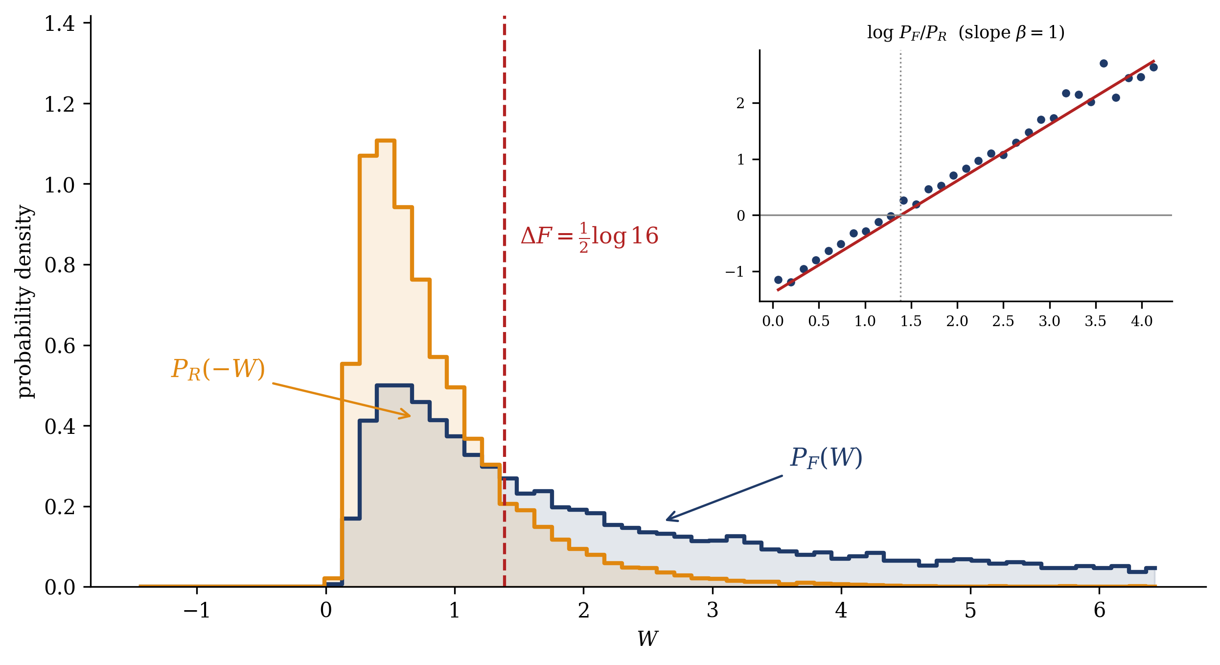
Figure 21.2 shows the Crooks theorem directly: at a moderate driving speed the forward work distribution \(P_F(W)\) and the reversed reverse-protocol distribution \(P_R(-W)\) intersect precisely at \(\Delta F\), and the log-ratio (inset) is a straight line of slope \(\beta = 1\), exactly as Equation 21.3 demands.
Figure 21.2: The Crooks crossing on the switched oscillator (stiffness \(1 \to 16\), \(\tau_s = 0.4\), \(N = 40\) increments, \(M = 15{,}000\) trajectories per direction). The forward work distribution \(P_F(W)\) (navy) dissipates and sits to the right; the reversed distribution \(P_R(-W)\) (orange) sits to the left; they intersect at the exact \(\Delta F = \tfrac12\log 16 \approx 1.386\) (red line), where the Crooks exponent \(\beta(W - \Delta F)\) vanishes. Inset: the log-ratio \(\log[P_F(W)/P_R(-W)]\) over the well-sampled region falls on a straight line of slope \(\beta = 1\) (red), the signature of Equation 21.3. The single-molecule experiments recover folding free energies from exactly this intersection.
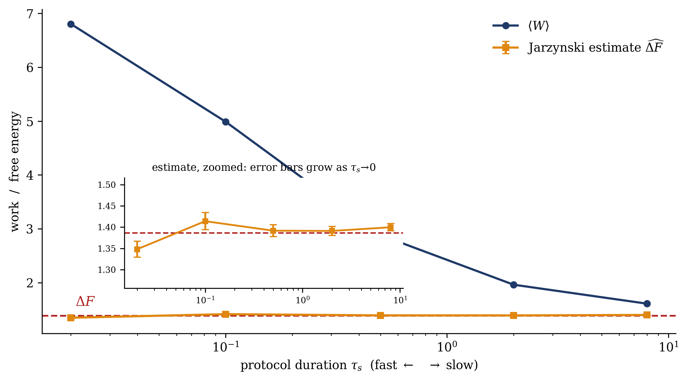
Figure 21.3 isolates the cost. As the protocol is driven faster, the mean work \(\langle W\rangle\) climbs well above \(\Delta F\) — that is the dissipation of Equation 21.5 growing — while the Jarzynski estimate Equation 21.6 sits on \(\Delta F\) at every speed. The equality is unbiased no matter how hard the drive. What speed costs, at this sample size, is variance: the bootstrap error bars widen as the driving accelerates, while the estimate itself holds on \(\Delta F\). There is a finite-sample bias too, and it is worth getting the sign right — it runs upward. The average \(\langle e^{-\beta W}\rangle\) is carried by rare low-work trajectories; a finite sample typically misses them, so the sample mean of \(e^{-\beta W}\) comes out too small and \(\widehat{\Delta F} = -\tfrac1\beta \log \overline{e^{-\beta W}}\) too large — Jensen’s inequality makes this a theorem, \(\mathbb{E}[\widehat{\Delta F}] \ge \Delta F\) (the Gore–Ritort–Bustamante bias). At \(M = 4000\) on this near-Gaussian oscillator that bias sits below the noise floor; it is what becomes severe under heavier-tailed driving, and exactly the failure annealed importance sampling exists to cure.
Show code
rng = np.random.default_rng(11)N, M =40, 4000taus = np.array([0.02, 0.1, 0.5, 2.0, 8.0])meanW, est, err = [], [], []for tau in taus: W = run_protocol(np.linspace(kA, kB, N +1), tau, M, rng) meanW.append(W.mean()) est.append(jarzynski(W)) boots = np.array([jarzynski(rng.choice(W, M)) for _ inrange(300)]) err.append(boots.std())fig, ax = plt.subplots(figsize=(8.0, 4.5))ax.plot(taus, meanW, "o-", color=NAVY, lw=1.8, ms=5, label=r"$\langle W\rangle$")ax.errorbar(taus, est, yerr=err, fmt="s-", color=ORANGE, lw=1.8, ms=5, capsize=3, label=r"Jarzynski estimate $\widehat{\Delta F}$")ax.axhline(dF, color=RED, lw=1.4, ls="--")ax.text(0.021, dF +0.18, r"$\Delta F$", color=RED, fontsize=11)ax.set_xscale("log")ax.set_xlabel(r"protocol duration $\tau_s$ (fast $\leftarrow$ $\rightarrow$ slow)")ax.set_ylabel("work / free energy")ax.legend(frameon=False, fontsize=10, loc="upper right")# inset: zoom on the estimate to reveal growing error bars toward fast drivingaxin = ax.inset_axes([0.13, 0.14, 0.44, 0.34])axin.errorbar(taus, est, yerr=err, fmt="s-", color=ORANGE, lw=1.5, ms=4, capsize=3)axin.axhline(dF, color=RED, lw=1.2, ls="--")axin.set_xscale("log"); axin.set_ylim(dF -0.13, dF +0.13)axin.set_title(r"estimate, zoomed: error bars grow as $\tau_s\!\to\!0$", fontsize=8.5)axin.tick_params(labelsize=7)fig.tight_layout(); plt.show()
Figure 21.3: Bias-free is not cost-free. Mean work \(\langle W\rangle\) (navy) and the Jarzynski free-energy estimate Equation 21.6 (orange, with bootstrap error bars) versus protocol duration \(\tau_s\), for the same \(1 \to 16\) switch (\(N = 40\), \(M = 4000\) trajectories, \(300\) bootstrap resamples). Slow driving (right) sits near equilibrium and \(\langle W\rangle \to \Delta F\); fast driving (left) dissipates, and \(\langle W\rangle\) rises far above the red reference \(\Delta F = \tfrac12\log 16\). The Jarzynski estimate holds on \(\Delta F\) across three decades of speed — the equality is exact at any \(\tau_s\) — while its error bars grow toward fast driving; the finite-sample bias runs upward (Jensen: \(\mathbb{E}[\widehat{\Delta F}] \ge \Delta F\)), from the ever-rarer low-work trajectories that carry the average, and stays below the noise floor at this \(M\).
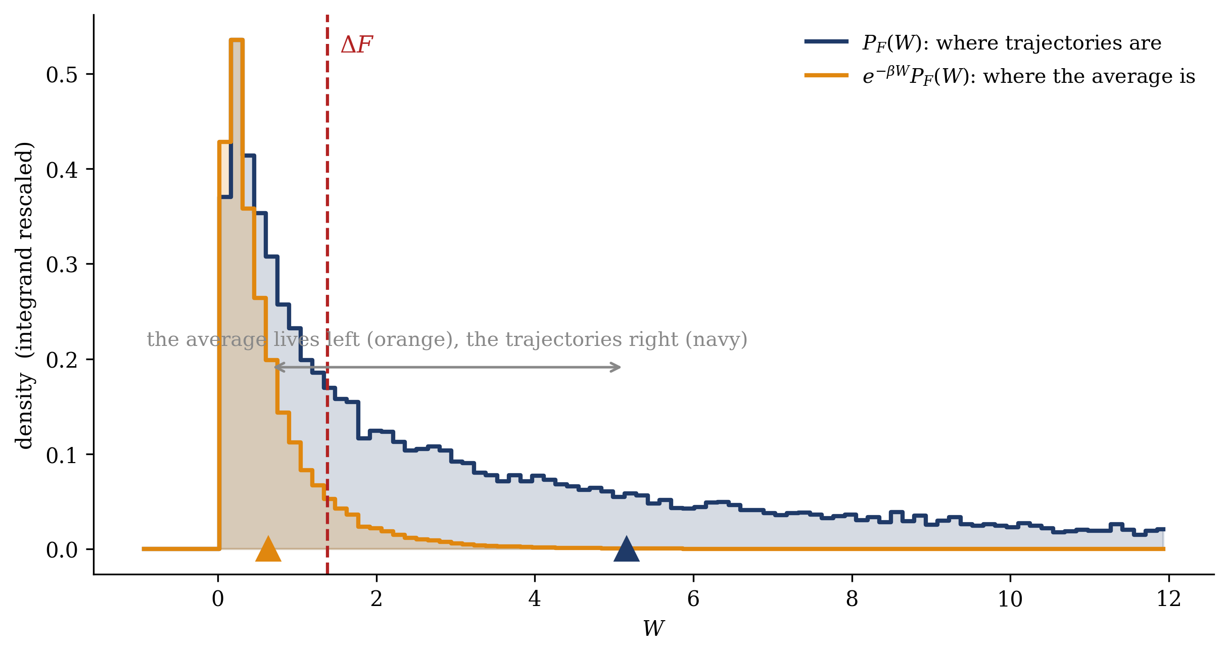
Finally, Figure 21.4 shows why strong driving makes the estimate fragile. It overlays the forward work distribution with the reweighted integrand \(e^{-\beta W}P_F(W)\) that the Jarzynski average actually integrates. Under fast driving the forward trajectories dissipate to a mean \(\langle W\rangle \approx 5\), far to the right of \(\Delta F\), but the reweighted integrand collapses onto the low-work trajectories near \(W \approx 0.5\): the estimator effectively discards the dissipated majority and leans on the low-work minority. For this near-Gaussian oscillator the imbalance is still manageable — which is why Figure 21.3 stays close to \(\Delta F\) — but the same mechanism, under a heavier-tailed protocol, is what makes the variance explode and forces the move to annealed importance sampling.
Show code
rng = np.random.default_rng(5)N, M, tau_s =40, 20000, 0.1Wf = run_protocol(np.linspace(kA, kB, N +1), tau_s, M, rng)edges = np.linspace(-1, 12, 90)c =0.5* (edges[:-1] + edges[1:])pf, _ = np.histogram(Wf, edges, density=True)w = np.exp(-Wf / T)meanW = Wf.mean()reweighted_meanW = (Wf * w).sum() / w.sum() # = <W e^{-bW}> / <e^{-bW}>integrand = np.exp(-c / T) * pfintegrand = integrand / integrand.max() * pf.max() # unit-peak rescale for displayfig, ax = plt.subplots(figsize=(8.2, 4.4))ax.fill_between(c, pf, step="mid", color=NAVY, alpha=0.18)ax.step(c, pf, where="mid", color=NAVY, lw=2.0, label=r"$P_F(W)$: where trajectories are")ax.fill_between(c, integrand, step="mid", color=ORANGE, alpha=0.20)ax.step(c, integrand, where="mid", color=ORANGE, lw=2.0, label=r"$e^{-\beta W}P_F(W)$: where the average is")ax.axvline(dF, color=RED, lw=1.5, ls="--")ymax = ax.get_ylim()[1]ax.text(dF +0.15, ymax *0.93, r"$\Delta F$", color=RED, fontsize=11)# mark the two means and the gap between themax.plot([meanW], [0], marker="^", color=NAVY, ms=11, clip_on=False)ax.plot([reweighted_meanW], [0], marker="^", color=ORANGE, ms=11, clip_on=False)ax.annotate("", xy=(meanW, ymax *0.34), xytext=(reweighted_meanW, ymax *0.34), arrowprops=dict(arrowstyle="<->", color=GRAY, lw=1.2))ax.text(0.5* (meanW + reweighted_meanW), ymax *0.38,"the average lives left (orange), the trajectories right (navy)", color=GRAY, fontsize=9.5, ha="center")ax.set_xlabel(r"$W$"); ax.set_ylabel("density (integrand rescaled)")ax.legend(frameon=False, fontsize=9.5, loc="upper right")fig.tight_layout(); plt.show()
Figure 21.4: Where the average lives. For a fast switch (\(\tau_s = 0.1\), \(M = 20{,}000\)), the forward work distribution \(P_F(W)\) (navy) dissipates: its mass stretches far to the right of \(\Delta F\) (red line), with mean \(\langle W\rangle\) (navy tick) well beyond it. But the Jarzynski average integrates the reweighted density \(e^{-\beta W}P_F(W)\) (orange, rescaled to unit peak for display), which by Crooks is proportional to \(P_R(-W)\) and collapses onto the low-work end, with reweighted mean (orange tick) near and below \(\Delta F\). The estimator is carried by the low-work minority and all but ignores the dissipated bulk it actually sampled — the origin of the variance that Section 21.4 flagged. For this near-Gaussian oscillator the mismatch is still mild; under stronger dissipation it is what annealed importance sampling exists to manage.
\(\langle e^{-\beta W}\rangle = e^{-\beta \Delta F}\) at any driving speed — equilibrium free energies, ratios of partition functions, bought with irreversible work; the second law is the Jensen shadow of an equality.
The tutorial (Ph12 106) is computation-led. You will verify the Jarzynski equality numerically on a system of your own and compute a free-energy difference by annealed importance sampling — the next lecture builds that algorithm from today’s ratio — and make explicit a connection this lecture has only named. The tutorial uses Equation 21.3, the work definition Equation 21.2, and the estimator Equation 21.6.
21.6 Outlook: from identity to algorithm
Today’s lecture converted \(\Delta F\) into a computable estimator. The partition function the course could not evaluate becomes, through Equation 21.1, a free-energy difference; the fluctuation theorems (Equation 21.3, Equation 21.4) compute that difference from finite-time, irreversible driving; and with a tractable reference the estimator Equation 21.6 delivers \(\log Z\) itself. To summarize the course’s treatment of \(Z\): \(Z\) was dodged in Module 1 (contrastive divergence), bounded in Module 2 (the variational free energy), cancelled in Module 3 (sampling), removed from training and generation in Week 10 (score matching and the reverse-time SDE), and now, as a ratio, measured.
What remains is engineering and assembly. The next lecture takes the estimator’s one weakness — variance that explodes with dissipation (Section 21.4) — and cures it by engineering the ladder of Section 21.2: many interpolating distributions with a detailed-balanced move on each rung, so that no single step dissipates much. That is annealed importance sampling (Neal (2001)), and its importance weights are exactly the \(e^{-\beta W}\) of Equation 21.6; it also closes the loop Week 8 opened, where annealing optimized and here the same construction measures. And Week 12 assembles the module’s machinery into the industrial object: diffusion models, whose training bound is a nonequilibrium free-energy estimator in precisely the sense derived today, and whose lineage runs straight back through Sohl-Dickstein et al. (2015) to the identities on this page. The reversal Week 10 proved exact has, as of today, a price — Equation 21.5 — and the whole of Module 4 is the account of paying it.
Collin, Delphine, Felix Ritort, Christopher Jarzynski, Steven B. Smith, Jr. Tinoco Ignacio, and Carlos Bustamante. 2005. “Verification of the Crooks Fluctuation Theorem and Recovery of RNA Folding Free Energies.”Nature 437 (7056): 231–34. https://doi.org/10.1038/nature04061.
Crooks, Gavin E. 1999. “Entropy Production Fluctuation Theorem and the Nonequilibrium Work Relation for Free Energy Differences.”Physical Review E 60 (3): 2721–26. https://doi.org/10.1103/PhysRevE.60.2721.
Liphardt, Jan, Sophie Dumont, Steven B. Smith, Jr. Tinoco Ignacio, and Carlos Bustamante. 2002. “Equilibrium Information from Nonequilibrium Measurements in an Experimental Test of Jarzynski’s Equality.”Science 296 (5574): 1832–35. https://doi.org/10.1126/science.1071152.
Sohl-Dickstein, Jascha, Eric Weiss, Niru Maheswaranathan, and Surya Ganguli. 2015. “Deep Unsupervised Learning Using Nonequilibrium Thermodynamics.” In Proceedings of the 32nd International Conference on Machine Learning, 37:2256–65. Proceedings of Machine Learning Research. https://arxiv.org/abs/1503.03585.
Welling, Max, Sirui Lu, and Lars Holdijk. 2026. Generative AI and Stochastic Thermodynamics: A Tale of Free Energies. Cambridge: Cambridge University Press. https://doi.org/10.1017/9781009709071.
Zwanzig, Robert W. 1954. “High-Temperature Equation of State by a Perturbation Method. I. Nonpolar Gases.”The Journal of Chemical Physics 22 (8): 1420–26. https://doi.org/10.1063/1.1740409.