Core (~1 h).Song, Sohl-Dickstein, et al. (2021) — the framework paper, and the warm-up reading (introduction and the SDE-framework section): one forward SDE, its stochastic reversal, and the probability-flow ODE that shares every marginal. The probability-flow section is today’s engine; the appendix derivations are worth a look after the lecture. Alongside it, re-read Ho, Jain, and Abbeel (2020) with today’s eyes: the variance-preserving SDE, discretized, with a particular loss weighting.
Optional background.Chen et al. (2018) — the instantaneous change of variables \(\tfrac{\mathrm{d}}{\mathrm{d}t}\log p = -\nabla \cdot v\) that makes the ODE’s likelihood exact, and the continuous-normalizing-flow lineage behind it. Grathwohl et al. (2019) — how the divergence is estimated at scale (the Hutchinson trace). Sohl-Dickstein et al. (2015) — the founding paper, one last time: everything today unifies descends from its forward/reverse construction. Lipman et al. (2023) — flow matching, the contemporaneous alternative that learns the deterministic velocity directly (skim). Karras et al. (2022) — the modern design-space view: schedule, scaling, and sampler as independent knobs (named today, not developed). Welling, Lu, and Holdijk (2026) — the companion text’s continuous-time and score-SDE chapters cover exactly this material.
Prerequisite reminder. From Week 10: the score \(\nabla_x \log p_t\) and its \(Z\)-freeness (Equation 19.1), denoising score matching (Equation 19.4 and Section 20.4), the forward noising process (Equation 20.1), and Anderson’s reverse-time SDE (Equation 20.2), whose Fokker–Planck derivation (Section 20.3) is re-run today with a different destination. From Week 9: the Fokker–Planck equation itself (Equation 17.3). From Week 11: the ELBO/AIS bound and its dissipation gap (Equation 22.4). From the previous lecture: DDPM — the discrete forward chain, the variational bound, and the \(\varepsilon\)-prediction loss. New content: the forward-SDE family and its VP/VE members, the probability-flow ODE derived from the Fokker–Planck equation, the exact likelihood by the instantaneous change of variables, and the unification of DDPM, NCSN, and the reverse SDE into one construction.
24.1 One model, three arbitrary choices
The previous lecture assembled the industrial object. DDPM fixes a forward Markov chain \(q(x_k \mid x_{k-1}) = \mathcal{N}\big(\sqrt{1 - \beta_k}\, x_{k-1},\, \beta_k\big)\) that corrupts data to noise in \(K\) discrete steps; trains a reverse chain by a variational bound (ELBO) on \(\log p\); and collapses that bound, after reparameterization, into \(\varepsilon\)-prediction — which is denoising score matching (Equation 19.4) at each noise level, in different units. The lecture closed on the structural identification that Week 11 prepared: the ELBO’s slack is a Kullback–Leibler divergence between the forward corruption path and the learned reversal — a dissipation, the same quantity that priced annealed importance sampling in Equation 22.4. A DDPM is a learned nonequilibrium transport, trained by minimizing its own dissipated work.
Today’s move is to notice how much of that construction is choice rather than law. DDPM fixes a discretization (a finite chain of \(K\) steps), a schedule (a particular sequence \(\beta_k\)), and a loss weighting (the “simple” \(\varepsilon\)-objective) — and, most consequentially, it only ever bounds the log-likelihood. Each choice can be stripped away, and Song, Sohl-Dickstein, et al. (2021) stripped all of them at once: underneath sits a single continuous object, a forward stochastic differential equation, whose reversal needs only the time-dependent score the model already learns. And the continuous object is more than tidier notation, because it admits not one way back but two. One is Anderson’s reverse-time SDE (Equation 20.2), stochastic and familiar from Week 10. The other is new, and it is the reason for this lecture: a deterministic ordinary differential equation with exactly the same time-marginals — and a deterministic invertible flow can do the one thing no ELBO can, namely compute its model’s log-likelihood exactly. The natural objection — how can a deterministic ODE and a noise-driven SDE possibly produce the same samples? — is the one the warm-up card poses. The answer is that they agree on every marginal\(p_t\) while disagreeing on every individual path, and a generative model is judged on marginals.
The history compresses two years of parallel invention. Sohl-Dickstein et al. (2015) built generation from nonequilibrium thermodynamics — destroy structure with a fixed diffusion, learn the reversal — and cited Jarzynski while doing it. Ho, Jain, and Abbeel (2020) made the construction work at scale, as the previous lecture’s DDPM. Independently, Song and Ermon (2019) reached generation through the score itself: networks fitted at a ladder of noise scales, sampled by annealed Langevin dynamics (Section 20.4). Song, Sohl-Dickstein, et al. (2021) showed these were a single framework seen through two discretizations, and added the exact likelihood that none of the predecessors had. The question, then: what is the schedule-free, discretization-free object beneath DDPM, and what does its deterministic reversal buy?
24.2 The forward-SDE family
Write the continuous forward process in full generality:
the forward-SDE family: one process, a schedule choice
run to a horizon \(T\) at which the marginal \(p_T\) is a tractable Gaussian. (Notation panel, once: \(T\) is the diffusion horizon, not a temperature, and \(W\) is a Wiener process again — Week 11’s work variable is retired, and \(\beta(t)\) below is a noise schedule, not an inverse temperature.) Two members of the family carry all the history. The variance-preserving (VP) choice takes \(f = -\tfrac{1}{2}\beta(t)\, x\) and \(g = \sqrt{\beta(t)}\): the drift shrinks every sample toward the origin at exactly the rate the noise inflates it, and \(p_T \to \mathcal{N}(0, I)\). Week 10’s workhorse (Equation 20.1) is the constant-schedule member \(\beta \equiv 2\). The variance-exploding (VE) choice takes \(f = 0\) and \(g = \sqrt{\mathrm{d}[\sigma^2(t)]/\mathrm{d}t}\): no shrinkage, noise piled on top of the data until it drowns them, \(p_T \to \mathcal{N}(0, \sigma_\mathrm{max}^2 I)\) — and this is precisely the noise ladder of Song and Ermon (2019), made continuous.
The claim that DDPM lives in this family is a two-line computation. Set \(\beta_k = \beta(t_k)\, \Delta t\) with step \(\Delta t = T/K\) and expand the previous lecture’s chain for small \(\Delta t\):
which is the Euler–Maruyama discretization of the VP-SDE, step by step. DDPM’s forward chain is not like a diffusion; it is the VP diffusion, sampled at \(K\) points. The marginals stay closed-form, as they must for denoising score matching to work: for the VP member, \(x_t \mid x_0 \sim \mathcal{N}\big(x_0\, e^{-B(t)/2},\, 1 - e^{-B(t)}\big)\) with \(B(t) = \int_0^t \mathrm{d}s\; \beta(s)\) — data convolved with a known Gaussian at every \(t\), exactly the setting of Section 20.4. One \(t\)-conditioned network \(s_\theta(x, t) \approx \nabla_x \log p_t(x)\), trained by denoising score matching across the whole continuum of times, is the single learned object in everything that follows.
The stochastic way back we already own. Anderson’s theorem (Equation 20.2), derived in Section 20.3 for exactly this family, reverses the forward SDE as
integrated from \(T\) down to \(0\): a stochastic generator, injecting fresh noise at every step, reproducing every marginal \(p_t\) exactly. So one process with marginals \(p_t\) runs forward, and a second, noise-driven one runs backward. The question the lecture turns on is whether a third process — deterministic, no \(\mathrm{d}\bar{W}\) at all — can carry the same marginals. If it can, it is an invertible map between noise and data, and invertible maps have exactly computable likelihoods. The answer is one rewrite of the Fokker–Planck equation away.
Take-home 1
DDPM is one instance of a continuous family: the forward SDE \(\mathrm{d}x = f\,\mathrm{d}t + g\,\mathrm{d}W\), with VP (\(f = -\tfrac{1}{2}\beta x\), \(g = \sqrt{\beta}\); DDPM is its Euler–Maruyama discretization) and VE (\(f = 0\); the NCSN noise ladder) as the two canonical schedules. One learned object serves the whole family — the time-marginal score \(s_\theta(x,t)\), fit by denoising score matching — and the reverse-time SDE is its stochastic way back. Today’s question: is there a deterministic way back with the same marginals?
24.3 The engine: Fokker–Planck as pure transport
We derive the deterministic generator in full; it runs entirely on Week 9’s machinery. Start from the marginal flow of the forward SDE, the Fokker–Planck equation of Equation 17.3 (scalar \(g(t)\) here; the matrix-valued case adds indices and nothing else):
The central step is a rewrite already used in Step 2 of the reversal argument in Section 20.3, where it served as scaffolding; here it is the result. The diffusion term is secretly a transport term: since \(\nabla_x p_t = p_t\, \nabla_x \log p_t\),
The display has a physical reading. A continuity equation\(\partial_t p = -\nabla \cdot (v p)\) is precisely the statement that probability is carried by the deterministic flow \(\dot{x} = v_t(x)\) — it is the Liouville transport equation of that ODE, the same bookkeeping that conserves phase-space density in classical mechanics. The display carries no trace of the velocity’s noisy origin. Therefore the ordinary differential equation with velocity \(v_t\) transports an initial density \(p_0\) through exactly the marginals \(p_t\) of the diffusion, and we box the master result (Song, Sohl-Dickstein, et al. 2021):
the probability-flow ODE — same marginals \(p_t\) as the forward and reverse SDE (Song et al. 2021)
In words: the diffusion term has been split in half — one half became deterministic transport, absorbed into the velocity as \(-\tfrac{1}{2} g^2 \nabla_x \log p_t\), and the other half was the injected noise, now removed entirely. Compare the drifts, because the factor of \(\tfrac{1}{2}\) is the central distinction: the reverse SDE carries the full\(g^2 \nabla_x \log p_t\) and re-injects noise; the probability-flow ODE carries half and injects nothing. The missing \(\tfrac{1}{2} g^2 \nabla_x \log p_t\) of drift is exactly compensated by the missing diffusion — same marginals, no randomness. Run backwards from \(x_T \sim p_T\), the ODE is a deterministic generator; run forwards from a data point, it is a deterministic encoder; and because it is a smooth, invertible flow, it is about to become a likelihood machine.
24.4 The exact likelihood
What does a density do along a deterministic flow? The continuity equation answers in one line. Divide \(\partial_t p = -(\nabla_x \cdot v)\, p - v \cdot \nabla_x p\) by \(p\):
the instantaneous change of variables (Chen et al. 2018)
The convective terms cancel, and what remains is the instantaneous change of variables(Chen et al. 2018): along the flow, the log-density changes at exactly the negative divergence of the velocity — where the flow compresses (\(\nabla \cdot v < 0\)), density rises; where it spreads, density falls. This is the continuous-time limit of the Jacobian determinant in an ordinary change of variables, accumulated infinitesimally instead of computed all at once. Integrate from \(0\) to \(T\), where the endpoint density \(p_T\) is the known Gaussian, and rearrange:
the exact model log-likelihood, by integrating the flow
with \(x(t)\) the probability-flow trajectory launched from \(x_0\). The recipe reads straight off the box: push the data point forward to noise along the ODE, accumulate the divergence of the velocity along the way, add the tractable Gaussian log-density at the far end — and the result is the exact log-likelihood of the model, not a bound on it. Normalization has kept this quantity out of reach since Week 1. The previous lecture’s ELBO under-reports \(\log p\) by its dissipation; Week 11’s AIS delivers a stochastic lower bound whose gap is the dissipated work (Equation 22.4); the probability-flow ODE closes the gap to zero, because a deterministic, invertible transport dissipates nothing. Three practical remarks belong in the record. In high dimension the divergence \(\nabla_x \cdot v\) is a trace of a \(d \times d\) Jacobian, estimated unbiasedly by the Hutchinson trace\(\nabla_x \cdot v = \langle \epsilon^\top (\partial_x v)\, \epsilon \rangle_{\epsilon \sim \mathcal{N}(0,I)}\) at the cost of one vector–Jacobian product (Grathwohl et al. 2019). The construction identifies the diffusion model as a continuous normalizing flow(Chen et al. 2018) whose velocity is fixed by the forward SDE and the learned score, rather than a free neural network. And there is a matching training-side result: a particular time-weighting of the denoising score-matching loss upper-bounds the negative log-likelihood, so the model can also be trained in likelihood units (Song, Durkan, et al. 2021) — named here, not derived.
Trap
The standard misreadings of the two reversals. ① Marginals, not paths — and mind the \(\tfrac{1}{2}\). The reverse-SDE drift carries \(f - g^2 \nabla_x \log p_t\) plus noise; the ODE velocity carries \(f - \tfrac{1}{2} g^2 \nabla_x \log p_t\) and no noise. The two agree on every distribution \(p_t\) and on no individual trajectory; copying the SDE drift into the ODE (or the reverse) is the standard algebra error. ② Exact is not the same as correct.Equation 24.2 is the exact likelihood of the model the learned score defines. With an imperfect \(s_\theta\) it can sit above or below the data’s true log-density — it is not a lower bound, and it inherits every flaw of the score. ③ The score needed is that of \(p_t\) for all \(t\) — Week 10’s trap, still load-bearing: the data score alone steers nothing out of noise. ④ DDPM, NCSN, and the score SDE are one model, not three.\(\varepsilon\)-prediction, the \(\sigma\)-scaled score, and \(\nabla_x \log p_t\) differ by fixed rescalings; VP versus VE is a schedule choice, not a framework choice. Treating them as rivals misreads the whole construction.
Take-home 2
Rewriting the Fokker–Planck equation as a continuity equation yields the probability-flow ODE (Equation 24.1): a deterministic flow with velocity \(v_t = f - \tfrac{1}{2} g^2 \nabla_x \log p_t\) that shares every marginal with the diffusion. Being an invertible flow, it computes the model’s log-likelihood exactly by the instantaneous change of variables (Equation 24.2) — where the ELBO and AIS only bound it, with a gap equal to their dissipation. Same marginals, different paths; note the \(\tfrac{1}{2}\).
24.5 The unification: Module 4 from four sides
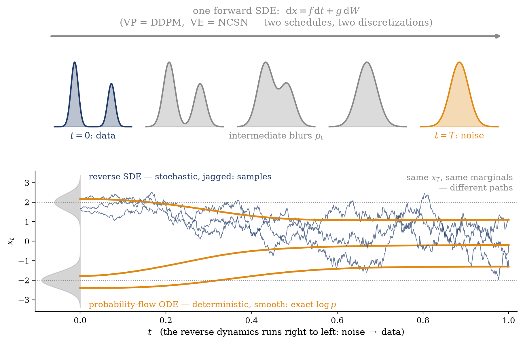
The module’s inventory can now be read off one construction, and Figure 24.1 is that reading as a picture. A diffusion model is a forward SDE \(\mathrm{d}x = f\,\mathrm{d}t + g\,\mathrm{d}W\) together with a single learned time-marginal score \(s_\theta(x, t)\). DDPM is the VP member, discretized by Euler–Maruyama, trained with one loss weighting; its ELBO is the discrete-time shadow of the continuous bound. NCSN and its annealed-Langevin sampler (Song and Ermon 2019) are the VE member: the ladder of noise scales is the VE schedule discretized, and annealed Langevin is a discretization of the reverse dynamics. Both are trained by denoising score matching across noise levels (Equation 19.4) — \(\varepsilon\)-prediction and \(\sigma\)-scaling are unit conversions on one objective. And from the same learned score there are two ways back: the reverse SDE (stochastic; fresh noise at each step partially corrects accumulated score error, which is why it tends to win on sample quality) and the probability-flow ODE (deterministic; fewer, larger steps; a bijective encoder; and the exact likelihood of Equation 24.2). Choose the sampler by purpose — the SDE for pictures, the ODE for numbers — and the choice is independent of schedule, architecture, and loss, which is the design-space decoupling that Karras et al. (2022) later made systematic.
Figure 24.1: The whole of Module 4 in one picture. Top: a single forward SDE carries the data density (navy) through blurred intermediates \(p_t\) (gray) to a tractable Gaussian (orange); DDPM and NCSN are its VP and VE schedules, discretized. Bottom: from the same terminal noise, two reversals driven by the same learned score — the stochastic reverse SDE (navy, jagged) and the deterministic probability-flow ODE (orange, smooth) — reproduce the same marginals along visibly different paths, and land on the same data density (gray, left edge). Trajectories computed with the exact score of the running two-mode example under a VP schedule.
The Week 11 thread ties off in one sentence, and the tutorial makes it concrete: a diffusion model is a learned annealed importance sampler — the forward SDE is the annealing ladder, the reverse dynamics the transport, the ELBO the Jarzynski-style path-KL bound of Equation 22.4 — with the probability-flow ODE supplying, at last, the exact number that AIS could only bound. And one contemporaneous development should be named. If the deterministic velocity field is the object that matters, one can regress a network onto it directly — flow matching (Lipman et al. 2023) fits \(v_\theta(x, t)\) to closed-form conditional velocities along prescribed interpolation paths, obtaining the transport without ever writing a stochastic process or a score. That the field’s newest mainline arrived by deleting the noise from the construction is a fair measure of how central the probability-flow view has become; conditional generation and guidance are further engineering on the same score field, and we leave them to the literature.
Take-home 3
Four Module-4 objects are one construction. The forward SDE (VP = DDPM, VE = NCSN) fixes the marginals; denoising score matching fits their score, whatever the parameterization; the reverse SDE and the probability-flow ODE are two samplers for the same model — stochastic for sample quality, deterministic for speed, encoding, and the exact likelihood; and the training bound is the dissipation of a learned annealed importance sampler (Week 11). Schedule, discretization, loss weighting, and sampler are independent knobs on one machine.
24.6 Example: two samplers and an exact likelihood
The framework’s three claims — same marginals, exact likelihood, bound strictly below — are all checkable on a target where nothing is learned and nothing is hidden. Take the two-mode mixture \(p_\mathrm{data} = 0.6\, \mathcal{N}(-2, 0.4^2) + 0.4\, \mathcal{N}(2, 0.4^2)\) under a VP forward SDE with linear schedule \(\beta(t) = 0.1 + 19.9\, t\) on \(t \in [0, 1]\). A Gaussian mixture stays a Gaussian mixture under the VP kernel, so the marginals \(p_t\), the score, and even the score’s spatial derivative are closed-form — the demonstration isolates the framework from learning error, exactly as in Section 20.5. We sample \(20{,}000\) points through both reversals (Euler–Maruyama for the SDE, a fixed-step Runge–Kutta integrator for the ODE), then compute the ODE likelihood Equation 24.2 at a grid of test points, and finally a DDPM-style ELBO on a \(K\)-step discretization of the same model.
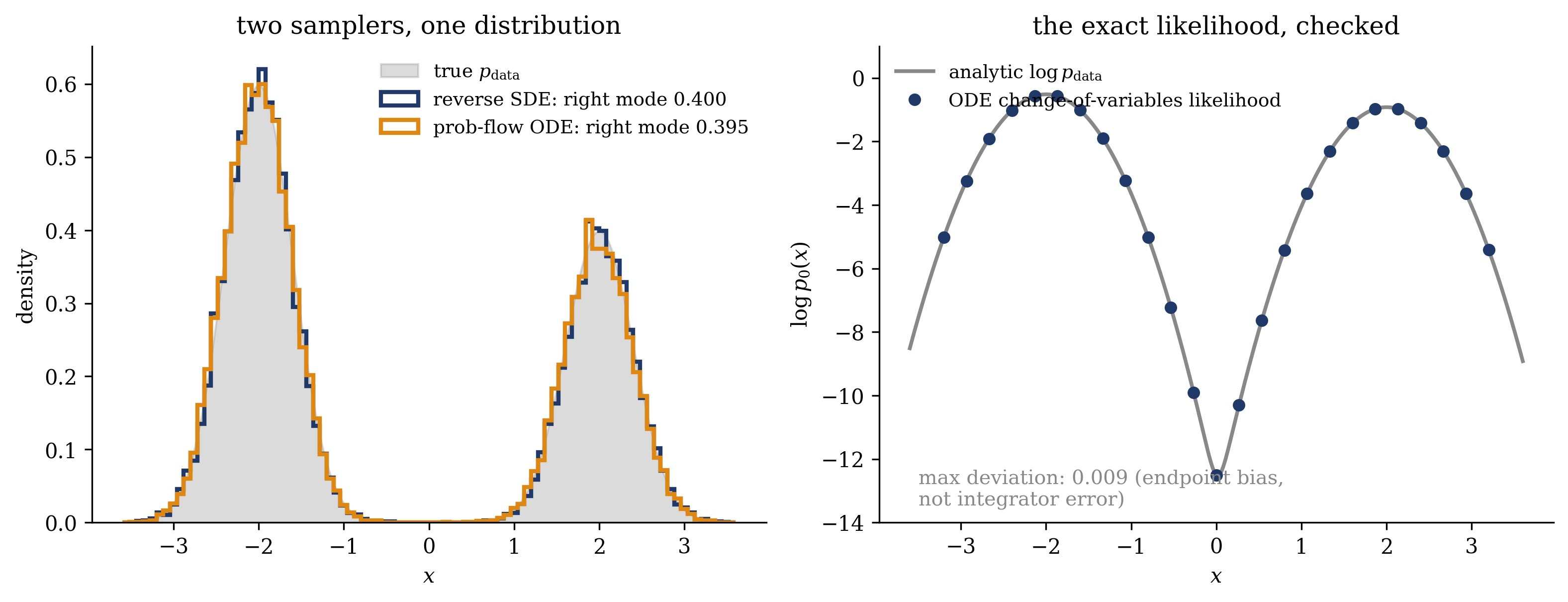
Figure 24.2: Two reversals of one diffusion, with the exact score (VP schedule, \(\beta(t) = 0.1 + 19.9\,t\); \(20{,}000\) samples each, common initial draws from \(\mathcal{N}(0,1)\)). Left: sample histograms from the reverse SDE (navy; Euler–Maruyama, \(1000\) steps) and the probability-flow ODE (orange; RK4, \(400\) steps) against the true data density (gray) — the measured right-mode weights are \(0.400\) and \(0.395\) against a true \(0.400\): same marginals, one stochastic path family and one deterministic. Right: the exact log-likelihood by the flow, Equation 24.2 — the ODE integrated forward from each test point with the divergence accumulated along the trajectory (navy dots) — against the analytic \(\log p_\mathrm{data}\) (gray curve). The agreement is a few times \(10^{-3}\); the visible residual is not integrator error but the endpoint bias \(p_T \neq \mathcal{N}(0,1)\) flagged in Section 20.2, here of order \(e^{-B(T)/2} \approx 7 \times 10^{-3}\).
The left panel of Figure 24.2 settles that objection with data: a noise-driven and a noiseless process, started from the same Gaussian draws, deliver the same distribution — down to the mode weights, which Week 10 showed is where samplers fail. The right panel is the key result: the divergence integral of Equation 24.2 lands on the analytic log-density across five orders of magnitude in probability, and its small residual has a physical name (the terminal marginal has not quite reached the unit Gaussian) rather than a statistical one. A deterministic transport produces a likelihood with zero variance, which no stochastic estimator can.
Show code
def elbo(x0, K, M=4000, seed=1):"""Stochastic ELBO of the K-step discretized reverse model at x0.""" rng = np.random.default_rng(seed) dt = T_END / K x = np.full(M, x0) lnw = np.zeros(M)for k inrange(K): t = k * dt b = beta(t) mean_f = x -0.5* b * x * dt # forward EM kernel xn = mean_f + np.sqrt(b * dt) * rng.normal(size=M) lnq =-0.5* (xn - mean_f)**2/ (b * dt) -0.5* np.log(2* np.pi * b * dt) t1 = t + dt # reverse EM kernel b1 = beta(t1) sc, _ = score_and_deriv(xn, t1) mean_r = xn - (-0.5* b1 * xn - b1 * sc) * dt lnp =-0.5* (x - mean_r)**2/ (b1 * dt) -0.5* np.log(2* np.pi * b1 * dt) lnw += lnp - lnq x = xn lnw +=-0.5* x**2-0.5* np.log(2* np.pi) # Gaussian prior at Treturn lnw.mean()x_pts = np.array([-2.4, -2.0, -1.6, 1.7, 2.3])truth = log_pt(x_pts, 0.0)elbo32 = np.array([elbo(x0, 32) for x0 in x_pts])Ks = np.array([8, 16, 32, 64, 128, 256])gaps = np.array([np.mean([log_pt(np.array([x0]), 0.0)[0] - elbo(x0, K)for x0 in x_pts]) for K in Ks])fig, (a1, a2) = plt.subplots(1, 2, figsize=(10.6, 4.0))xs = np.linspace(-3.3, 3.3, 400)a1.plot(xs, log_pt(xs, 0.0), color=GRAY, lw=1.8, label=r"analytic $\log p_\mathrm{data}$")a1.plot(x_pts, truth, "o", color=NAVY, ms=6, label="prob-flow ODE (exact)")a1.plot(x_pts, elbo32, "s", color=ORANGE, ms=6, label=r"ELBO, $K = 32$ steps")for xp, tv, ev inzip(x_pts, truth, elbo32): a1.plot([xp, xp], [ev, tv], color=ORANGE, lw=1.0, alpha=0.6)a1.annotate("gap = dissipation (W11)", xy=(-1.6, 0.5* (truth[2] + elbo32[2])), xytext=(-0.3, 0.35), ha="center", color=GRAY, fontsize=9.5, arrowprops=dict(arrowstyle="->", color=GRAY, lw=1.1))a1.set_xlabel(r"$x$"); a1.set_ylabel(r"$\log p_0(x)$")a1.set_ylim(-8, 1)a1.set_title("the bound sits below the number", fontsize=12)a1.legend(frameon=False, fontsize=9, loc="lower center")a2.plot(Ks, gaps, "o-", color=NAVY, lw=1.8, ms=5, label="mean ELBO gap")a2.plot(Ks, gaps[-1] * Ks[-1] / Ks, "--", color=ORANGE, lw=1.6, label=r"$\propto 1/K$ guide")a2.set_xscale("log", base=2); a2.set_yscale("log")a2.set_xlabel(r"chain length $K$"); a2.set_ylabel("ELBO gap (nats)")a2.set_title("refining the chain closes the gap", fontsize=12)a2.legend(frameon=False, fontsize=9)fig.tight_layout()plt.show()
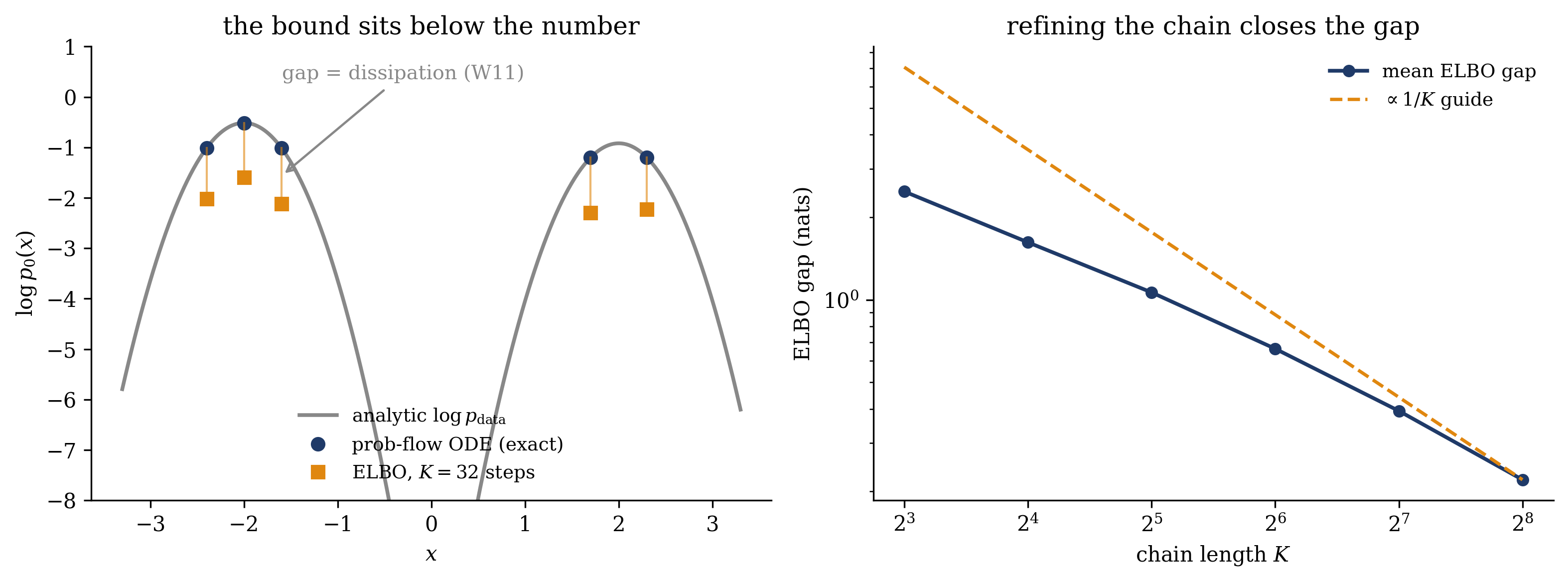
Figure 24.3: The bound and the number. Left: at five in-support test points, the \(K\)-step DDPM-style ELBO (orange: \(K = 32\); \(4000\) forward paths per point, EM reverse kernels built from the exact score) sits strictly below the analytic \(\log p_\mathrm{data}\) (gray curve), which the deterministic flow reproduces exactly (navy dots); the vertical offset is the discretization’s dissipated work, \(D_\mathrm{KL}(q_F \| q_R)\) of Equation 22.4. Right: the mean ELBO gap against the chain length \(K\), with a \(1/K\) guide (dashed) — refining the discretization recovers the continuum and the bound tightens toward the exact value, the near-equilibrium law of Section 22.5 operating inside a diffusion model.
Figure 24.3 makes the comparison quantitative. At \(K = 32\) steps the DDPM-style bound under-reports the log-likelihood by about one nat at every test point — that offset is the dissipation of the discrete transport, Week 11’s Jensen gap produced inside a diffusion model — and lengthening the chain shrinks it toward the \(1/K\) law that priced annealed importance sampling in Section 22.5. The deterministic flow stands outside this accounting: it sits on the exact value at any budget, because it never dissipates. Bound, dissipation, and exact number are on one plot, and they are the same three objects the course met as the second law, the dissipated work, and the free energy.
One forward SDE, one learned score, two ways back — a noisy reverse SDE for samples and a deterministic ODE for the exact likelihood; DDPM and score matching were the same model, discretized two ways.
The tutorial (16–18, Ph12 106) is derivation-led, and it closes the module’s practical arc: train a small score network on a two-dimensional density, sample it through both reversals, and compute its exact log-likelihood by the probability-flow ODE — the learned counterpart of everything the example above did with closed-form scores. The session uses Equation 24.1 and the change-of-variables identity, and ends by identifying the Week-11 ancestor of the training loss.
24.7 Outlook: the title, discharged
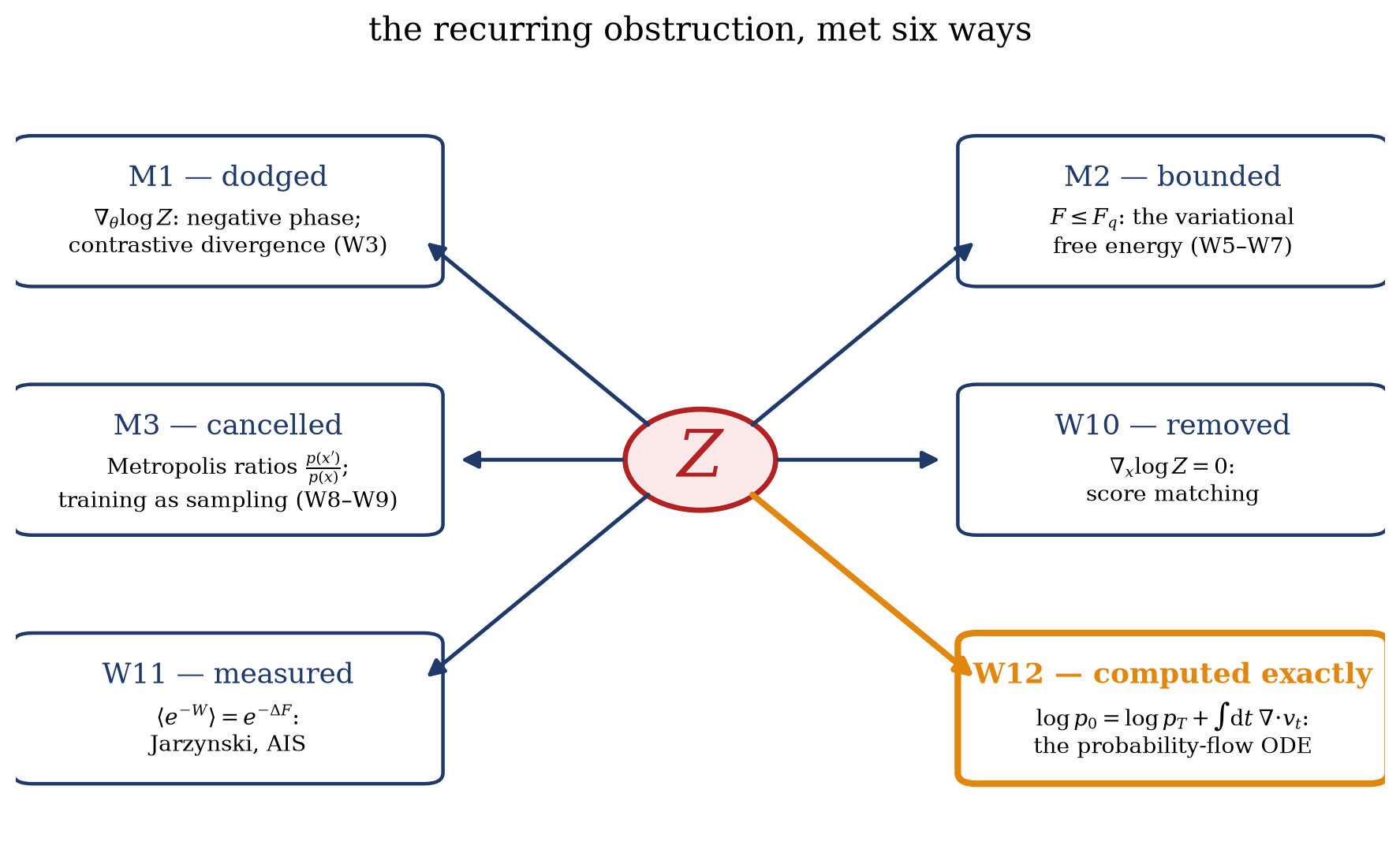
Week 12 closes the course’s main construction. The partition function was raised as the central obstruction in Week 1 and has organized every module since: Module 1 dodged its gradient with contrastive divergence, Module 2 bounded it with the variational free energy, Module 3 cancelled it inside Metropolis ratios, Week 10 removed it from training and generation outright, and Week 11 measured it with nonequilibrium work. This week the generative model built on the \(Z\)-free score reported its own log-likelihood exactly (Equation 24.2), and Figure 24.4 closes the figure the course has been extending since Figure 19.4. The chain of identifications runs from Boltzmann’s \(e^{-E}/Z\) to a diffusion model’s reverse-time flow: the energy defined a score, the score defined a drift, the drift defined a transport, and the transport’s divergence integral yields the likelihood.
Figure 24.4: The course’s spine, discharged. The partition function, met six ways: dodged (M1), bounded (M2), cancelled (M3), removed (W10), measured (W11) — and finally, this week, made irrelevant to the one question it always blocked: the model built on the \(Z\)-free score computes its own log-likelihood exactly, through the probability-flow ODE.
Two weeks remain, and they turn the machinery back on learning itself. Week 13 leaves generative modeling for the return direction of the bridge: its first lecture casts maximum entropy and the information bottleneck as constrained free-energy minimizations — the same variational language, applied to representation and compression rather than generation, with a precise account of what that framework establishes about deep networks and what it does not — and its second puts a partition function on the hypotheses of an inference problem, where sharp detectability thresholds separate the recoverable from the impossible, and a further threshold separates what is possible from what is efficiently achievable. That lecture does something the course has not done before: it uses statistical physics to decide what a learning problem admits, rather than to supply a method for one. Week 14 then reads all five modules off a single variational identity, prepares the exam, and surveys the research programme Week 13’s material is drawn from (Zdeborová and Krzakala 2016). On the generative side the onward reading is the flow-matching line named above (Lipman et al. 2023), together with Schrödinger bridges and the optimal-transport view of diffusion, for which the companion text (Welling, Lu, and Holdijk 2026) is the natural start. The construction ends here; what follows uses it on questions of a different kind.
Chen, Ricky T. Q., Yulia Rubanova, Jesse Bettencourt, and David Duvenaud. 2018. “Neural Ordinary Differential Equations.” In NeurIPS, 31:6572–83.
Grathwohl, Will, Ricky T. Q. Chen, Jesse Bettencourt, Ilya Sutskever, and David Duvenaud. 2019. “FFJORD: Free-Form Continuous Dynamics for Scalable Reversible Generative Models.” In ICLR.
Ho, Jonathan, Ajay Jain, and Pieter Abbeel. 2020. “Denoising Diffusion Probabilistic Models.” In Advances in Neural Information Processing Systems. Vol. 33. https://arxiv.org/abs/2006.11239.
Karras, Tero, Miika Aittala, Timo Aila, and Samuli Laine. 2022. “Elucidating the Design Space of Diffusion-Based Generative Models.” In NeurIPS. Vol. 35.
Lipman, Yaron, Ricky T. Q. Chen, Heli Ben-Hamu, Maximilian Nickel, and Matt Le. 2023. “Flow Matching for Generative Modeling.” In ICLR.
Sohl-Dickstein, Jascha, Eric Weiss, Niru Maheswaranathan, and Surya Ganguli. 2015. “Deep Unsupervised Learning Using Nonequilibrium Thermodynamics.” In Proceedings of the 32nd International Conference on Machine Learning, 37:2256–65. Proceedings of Machine Learning Research. https://arxiv.org/abs/1503.03585.
Song, Yang, Conor Durkan, Iain Murray, and Stefano Ermon. 2021. “Maximum Likelihood Training of Score-Based Diffusion Models.” In NeurIPS. Vol. 34.
Song, Yang, and Stefano Ermon. 2019. “Generative Modeling by Estimating Gradients of the Data Distribution.” In Advances in Neural Information Processing Systems (NeurIPS). Vol. 32.
Song, Yang, Jascha Sohl-Dickstein, Diederik P. Kingma, Abhishek Kumar, Stefano Ermon, and Ben Poole. 2021. “Score-Based Generative Modeling Through Stochastic Differential Equations.” In International Conference on Learning Representations. https://arxiv.org/abs/2011.13456.
Welling, Max, Sirui Lu, and Lars Holdijk. 2026. Generative AI and Stochastic Thermodynamics: A Tale of Free Energies. Cambridge: Cambridge University Press. https://doi.org/10.1017/9781009709071.
Zdeborová, Lenka, and Florent Krzakala. 2016. “Statistical Physics of Inference: Thresholds and Algorithms.”Advances in Physics 65 (5): 453–552. https://doi.org/10.1080/00018732.2016.1211393.