25The information bottleneck: representation at a temperature
Recommended reading
Core (~1 h).Tishby, Pereira, and Bialek (1999) — four pages of statistical physics under an information-theory title, and the warm-up reading for the next lecture: the rate–relevance Lagrangian, its variational solution, and the self-consistent equations that are today’s engine. Read §2–3 knowing what to look for: a Boltzmann distribution, a partition function, and a Lagrange multiplier that is an inverse temperature. Alongside it, the rate–distortion section of Shannon (1948) — where “bits spent describing \(X\)” acquires its precise meaning, and the frame the bottleneck generalizes.
Optional background.Rose (1998) — deterministic annealing and the phase transitions of rate–distortion, the physics reading of today’s material worked out a decade before the bottleneck paper; Alemi et al. (2017) — the trainable version, whose variational bound is Week 7’s ELBO with a predictive target; Tishby and Zaslavsky (2015) and Shwartz-Ziv and Tishby (2017) — the claim that deep networks themselves traverse the information plane, and Saxe et al. (2018) — its rebuttal, the pair to be read together; Friston (2010) — the free-energy principle, the most ambitious extension of this module’s language, read for the claim and its critique rather than as settled theory.
Prerequisite reminder. The Boltzmann distribution, \(Z\), \(\beta = 1/T\), and \(F = -T \ln Z\) (Equation 1.2); entropy and information in nats, and Jaynes’ maximum-entropy route to the canonical ensemble (Section 1.4); the variational free energy and the KL divergence as a free-energy difference (Equation 9.1); the ELBO and amortized inference (Equation 14.5, Equation 14.6); annealing as a cooling schedule (Chapter 16); the mean-field self-consistent equations (Equation 9.3). New content: the rate–relevance trade-off and the information plane, the bottleneck Lagrangian and its self-consistent equations, the free-energy reading with \(\beta\) as an inverse temperature, the structural phase transitions of the representation, the deep variational bottleneck, and the free-energy principle stated critically.
25.1 A constraint completes the principle
Week 12 closed the course’s main construction, and Module 5 — this week, plus the synthesis of Week 14 — widens the view. Before the machinery is put away, we ask how far its central principle reaches, and the principle in question is the variational one. Three times the course has met it. Jaynes’ maximum-entropy argument (Section 1.4) produced the Boltzmann distribution by maximizing entropy at fixed mean energy — a constrained optimization whose Lagrange multiplier turned out to be the inverse temperature. The Gibbs–Bogoliubov identity (Equation 9.1) turned inference into minimization: the variational free energy exceeds the true one by exactly \(T\, D_\mathrm{KL}(q \| p)\), so approximating a distribution and minimizing a free energy are the same act. And Week 7 trained that act, with the VAE descending the same functional by stochastic gradients (Equation 14.6). What none of these answers is a question that sits upstream of all of them: what should a representation be? A latent code, a layer’s activations, a clustering, a sufficient statistic — every learned system keeps some aspects of its input and discards the rest, and the free-energy principle as stated so far offers no criterion for the choice.
The criterion, due to Tishby, Pereira, and Bialek (1999), falls out of the same principle once a constraint is attached. Pose learning, at its most general, as lossy compression toward a goal: given an input \(X\) and a target \(Y\), find a compressed description \(\tilde{X}\) of \(X\) that keeps what predicts \(Y\) and discards everything else. This is not the autoencoder’s task — Week 7 asked \(\tilde{X}\) to reconstruct \(X\) itself — but the sharper one of keeping only what matters, with “matters” defined by the prediction target. Shannon supplies the two measures. The rate\(I(X;\tilde{X})\) counts the nats the description spends on \(X\); the relevance\(I(\tilde{X};Y)\) counts the nats it retains about \(Y\); and the compressed variable is required to see the target only through the input, the Markov chain \(X \rightarrow \tilde{X} \rightarrow Y\). The two measures are coupled. Zero rate forces zero relevance, since a description carrying no information about \(X\) carries none about anything downstream of it; the identity map \(\tilde{X} = X\) keeps every relevant nat and every irrelevant one with it. The interesting encoders live between the extremes, and the information bottleneck is the principle that selects them: minimize the rate while maximizing the relevance, at an exchange rate \(\beta\) whose interpretation as an inverse temperature the derivation of Section 25.3 establishes.
Shannon (1948) defined the rate–distortion function — the least rate at which a source can be described without exceeding a prescribed distortion — but left the distortion measure to be chosen by hand, and the choice always smuggled in the answer to “what matters.” Tishby, Pereira, and Bialek (1999) removed the hand: let the prediction task itself define the distortion, and the trade-off becomes intrinsic. The statistical mechanics predated the bottleneck paper — Rose (1998), reviewing a programme begun a decade earlier, had worked out rate–distortion theory as an equilibrium system, with the trade-off multiplier an inverse temperature and the optimal code reorganizing through genuine phase transitions as it cools. The identification below runs in the bottleneck’s setting, and Alemi et al. (2017) turns the result into a trainable network (Section 25.5). The next lecture takes the phase-transition thread and makes it the topic; Week 14 states the whole course as one functional.
25.2 Rate, relevance, and the information plane
We fix notation first, because the bottleneck literature has a trap in it. The compressed variable is written \(\tilde{X}\) throughout — as in Tishby, Pereira & Bialek’s original paper; the deep-learning-era bottleneck literature calls it \(T\), and we decline to follow it, since \(T\) has meant temperature for twelve weeks and is about to mean temperature again in the same equation. Both mutual informations are functionals of one object, the stochastic encoder\(p(\tilde{x} \mid x)\):
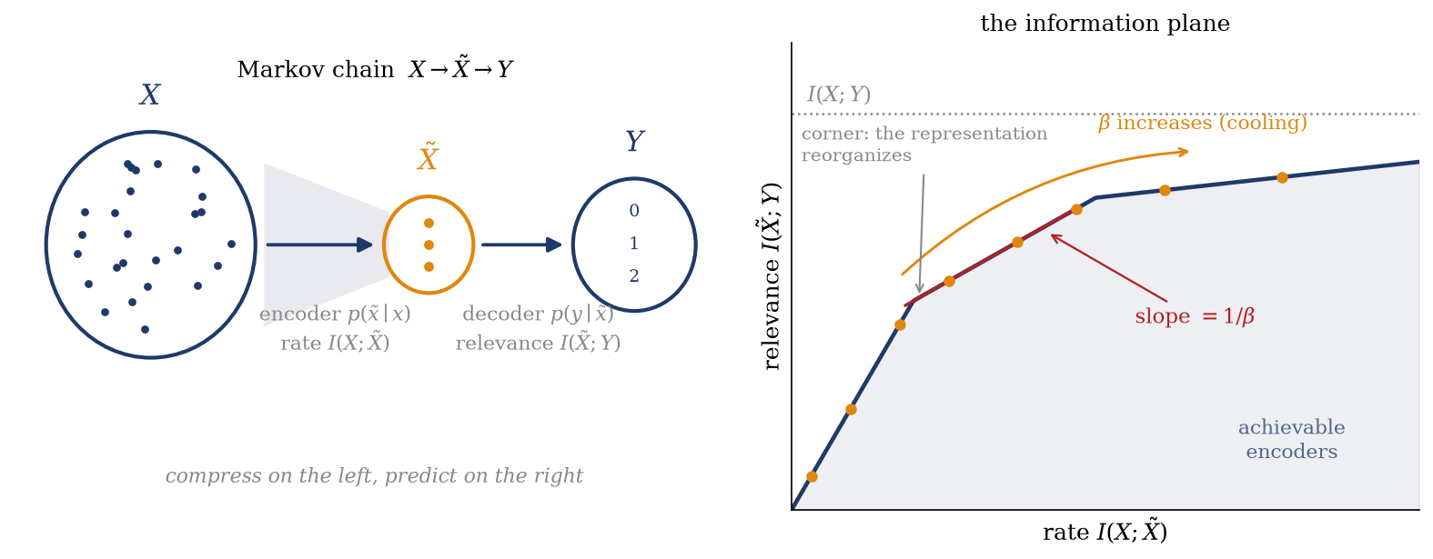
where the marginal \(p(\tilde{x}) = \sum_x p(x)\, p(\tilde{x} \mid x)\) and the joint \(p(\tilde{x}, y) = \sum_x p(x, y)\, p(\tilde{x} \mid x)\) are both induced by the encoder — the second equality using the Markov property, since \(\tilde{x}\) learns about \(y\) only through \(x\). Every possible encoder therefore maps to a point \((I(X;\tilde{X}),\, I(\tilde{X};Y))\) in the information plane, drawn in Figure 25.1: rate on the horizontal axis, relevance on the vertical. Two bounds fence the achievable region. The data-processing inequality caps relevance at the total \(I(X;Y)\) — no processing of \(X\) can know more about \(Y\) than \(X\) does — and relevance can never exceed rate, the same inequality read along the chain \(Y \to X \to \tilde{X}\) (the encoder cannot pack more about \(Y\) into \(\tilde{X}\) than the bits it spends describing \(X\)). The achievable points fill a region whose upper boundary, the IB curve, is the object of the lecture: the most relevance obtainable at each rate, concave, rising steeply from the origin and saturating toward \(I(X;Y)\).
Figure 25.1: The central picture of the lecture. Left: the Markov chain \(X \rightarrow \tilde{X} \rightarrow Y\), pinched at the compressed variable — the encoder spends rate \(I(X;\tilde{X})\) describing the input, the decoder keeps relevance \(I(\tilde{X};Y)\) about the target. Right: the information plane. Every encoder is a point; the achievable region (shaded) is bounded above by the concave IB curve, whose local slope is \(1/\beta\) — the temperature. Increasing \(\beta\) cools the encoder up the frontier, and at discrete corners the optimal representation reorganizes; the worked example of Section 25.6 computes this curve, corners included, for a small joint distribution.
Optimal encoders sit on the frontier, and the standard device converts the constrained problem — maximize \(I(\tilde{X};Y)\) at fixed rate — into an unconstrained one. Introducing a Lagrange multiplier \(\beta\) for the constraint gives the information-bottleneck Lagrangian,
to be minimized over all normalized conditionals \(p(\tilde{x} \mid x)\). The signs are not interchangeable, because flipping them inverts the whole construction: the rate is the cost and enters with a plus, the relevance is the benefit and is subtracted with weight \(\beta\). Geometrically, \(\beta\) selects the operating point: minimizing Equation 25.1 at a given \(\beta\) picks the point of the frontier where the tangent slope \(\mathrm{d}I(\tilde{X};Y)/\mathrm{d}I(X;\tilde{X})\) equals \(1/\beta\). Small \(\beta\) weights compression heavily and lands near the steep origin, where the first nats of rate buy relevance cheaply; large \(\beta\) demands fidelity and rides the flat tail toward saturation, where each additional nat of relevance costs many nats of rate. The slope of the frontier, in other words, behaves exactly like a temperature \(1/\beta\). Jaynes’ construction (Section 1.4) already showed that a multiplier enforcing a constraint on an entropy-like quantity is an inverse temperature; the bottleneck inherits the identification, and the derivation of the next section makes it literal, partition function included.
Two remarks precede the calculus. First, minimizing Equation 25.1 is a variational problem, not an ordinary optimization: the unknown is an entire conditional distribution, one probability vector for every input \(x\), and both terms depend on it also implicitly, through the induced \(p(\tilde{x})\) and \(p(\tilde{x}, y)\). Second, \(\beta\) is our old symbol with its old meaning restored. It was the inverse temperature of Week 1, was flagged against the ML community’s unrelated uses (the Adam moments, the β-VAE weight), and spent Week 12 as a noise schedule \(\beta_t\) (Section 23.2); here it returns as a genuine \(1/T\), and the identification is completed in Section 25.3, where a partition function appears beside it.
Take-home 1
Learning, posed at its most general, is lossy compression toward a target: over the Markov chain \(X \rightarrow \tilde{X} \rightarrow Y\), minimize the rate \(I(X;\tilde{X})\) while maximizing the relevance \(I(\tilde{X};Y)\). The achievable encoders fill a region of the information plane bounded by the concave IB curve, and the Lagrangian \(\mathcal{L} = I(X;\tilde{X}) - \beta\, I(\tilde{X};Y)\) (Equation 25.1) selects the frontier point of slope \(1/\beta\) — the multiplier is an exchange rate between nats spent and nats predicted, and, as with Jaynes’ maximum entropy, it will prove to be an inverse temperature.
25.3 The engine: stationarity of the Lagrangian
What encoder makes Equation 25.1 stationary? The answer’s form is the bridge to statistical mechanics, so we carry the variation out in full. Write the Lagrangian with its normalization constraints attached,
and differentiate with respect to one entry \(p(\tilde{x} \mid x)\), at fixed \((x, \tilde{x})\). The one technical point of the derivation — Theorem 4 of Tishby, Pereira, and Bialek (1999) — is that the induced objects must be differentiated too: \(p(\tilde{x})\) and \(p(\tilde{x}, y)\) both move when the encoder does, with \(\delta p(\tilde{x})/\delta p(\tilde{x} \mid x) = p(x)\) and \(\delta p(\tilde{x}, y)/\delta p(\tilde{x} \mid x) = p(x)\, p(y \mid x)\). Carrying both dependences through, the rate term gives
the two dangling \(+1\)’s cancelling. For the relevance term, expand \(I(\tilde{X};Y) = \sum p(\tilde{x}, y) \ln p(\tilde{x}, y) - \sum_{\tilde{x}} p(\tilde{x}) \ln p(\tilde{x}) - \sum_y p(y) \ln p(y)\) and note that the last sum does not involve the encoder at all. The same bookkeeping then yields
where the second step adds and subtracts \(\beta \sum_y p(y \mid x) \ln p(y \mid x)\) — a quantity that does not depend on \(\tilde{x}\) and can therefore be absorbed into the normalization. This is the central step, because what it isolates is a Kullback–Leibler divergence: the effective distortion\(d(x, \tilde{x}) = D_\mathrm{KL}\big[ p(y \mid x) \,\|\, p(y \mid \tilde{x}) \big]\), measuring how badly the decoder attached to representation \(\tilde{x}\) predicts the target compared to the input itself. Nobody chose this distortion; the variation manufactured it from the prediction task. Exponentiating and normalizing, we box the master result:
The optimal soft assignment of input \(x\) to representation \(\tilde{x}\) is a Boltzmann distribution — the prior \(p(\tilde{x})\) tilted by \(e^{-\beta d}\) — whose energy is the prediction error of \(\tilde{x}\)’s decoder on \(x\)’s conditional, whose temperature \(1/\beta\) sets how softly the assignment commits, and whose normalizer \(Z(x, \beta)\) is a partition function, one per input. The second and third equations close the system: the marginal is induced by the encoder, and the decoder is the Bayes rule of the encoder. All three are coupled — the energy in the first equation is computed against the decoder of the third, which is built from the encoder of the first — so Equation 25.2 is a fixed point to be reached by iteration.
Before the free-energy reading, one identity confirms that the manufactured distortion is the canonical one. Averaging \(d\) over the joint and splitting the logarithm,
the mean distortion is exactly the relevance lost in compression, nat for nat, so maximizing relevance and minimizing this particular distortion are the same act. With \(d\) in hand, the whole Lagrangian acquires a thermodynamic form. A short rearrangement using this identity and \(I(X;\tilde{X}) = \sum_x p(x)\, D_\mathrm{KL}[p(\tilde{x} \mid x) \| p(\tilde{x})]\) gives, for any encoder,
and the braced quantity is a free energy: mean energy plus temperature times a relative entropy, \(F = \langle E \rangle - TS\) with the entropy measured relative to the prior \(p(\tilde{x})\). Minimizing it over the encoder of one input, at fixed marginal and decoder, is the Gibbs variational problem of Section 1.4, and its solution and minimum are the ones every partition function announces:
attained precisely by the Boltzmann encoder of Equation 25.2. Since \(I(X;Y)\) is a constant of the problem, minimizing the IB Lagrangian is minimizing the mean of these per-input free energies, \(\bar{F}(\beta) = \sum_x p(x)\, f(x, \beta)\) — the central identity. The Boltzmann distribution of Week 1 is the encoder of Week 13, and representation learning is constrained free-energy minimization.
Take-home 2
The IB Lagrangian is stationary at \(p(\tilde{x} \mid x) = \frac{p(\tilde{x})}{Z(x, \beta)}\, e^{-\beta\, d(x, \tilde{x})}\) with \(d(x, \tilde{x}) = D_\mathrm{KL}[p(y \mid x) \| p(y \mid \tilde{x})]\), coupled to the induced marginal and the Bayes decoder (Equation 25.2). The distortion is manufactured by the variation, not chosen, and its mean equals the relevance lost; the normalizer \(Z(x, \beta)\) is a partition function whose free energy \(-\frac{1}{\beta} \ln Z\) (Equation 25.3) the optimal encoder minimizes. The optimal representation is the Boltzmann distribution of a rate–distortion free energy.
25.4 A temperature for representation
The two limits of \(\beta\) now read as the two limits of any thermal system. As \(\beta \rightarrow 0\) — infinite temperature — the exponential in Equation 25.2 flattens toward one, the encoder relaxes onto the prior, \(p(\tilde{x} \mid x) \rightarrow p(\tilde{x})\) for every input, and a single effective description swallows the whole source: \(I(X;\tilde{X}) = I(\tilde{X};Y) = 0\), the origin of the information plane. As \(\beta \rightarrow \infty\) — zero temperature — the assignment freezes onto the distortion’s ground state, each \(x\) committing deterministically to its best representation; the encoder becomes a hard partition, the relevance saturates toward \(I(X;Y)\), and in the limit \(\tilde{X}\) approaches a minimal sufficient statistic of \(X\) for \(Y\), the coarsest description that predicts as well as the data allow. Between the limits, sweeping \(\beta\) upward traces the IB curve from the compressed end to the faithful end, and doing the sweep gradually — solving at one \(\beta\), then warm-starting the next from the converged solution — is deterministic annealing(Rose 1998), the cooling of Chapter 16 repurposed from optimization to representation.
The cooling is not smooth, and this is the observation the next lecture will generalize. At high temperature the one-cluster solution is a genuine fixed point of Equation 25.2, and one can ask when it stops being stable: perturbing the uniform encoder and linearizing the update, the perturbation grows once \(\beta\) exceeds a critical value set by the leading eigenvalue of a covariance-like operator built from the conditionals \(p(y \mid x)\) — inputs whose conditionals align push the same direction, and the most self-reinforcing direction condenses first (Rose 1998). At that \(\beta_c\) the single description splits in two; further critical temperatures split the daughters in turn; and the number of distinct representations in use climbs a staircase as the system cools. These are structural phase transitions in the precise sense of Week 5 — a symmetry of the solution breaking at a critical temperature, the order parameter now information-theoretic — and between them the representation is qualitatively rigid: cooling sharpens the assignments but does not reorganize them. On the IB curve the transitions appear as the corners of Figure 25.1, where the frontier’s slope changes discontinuously; the worked example below computes the staircase and both of its critical temperatures on a system small enough to watch.
The algorithm falls out of the equations’ own structure. Since each of the three relations in Equation 25.2 is the exact optimum given the other two, alternate them: ① update the encoder from the current marginal and decoder by the Boltzmann rule, ② update the marginal from the new encoder, ③ update the decoder by Bayes. Each sweep lowers \(\mathcal{L}\) monotonically, and the iteration converges to a fixed point — this is the Blahut–Arimoto algorithm of rate–distortion theory, transplanted. The same alternating self-consistency appeared in the mean-field equations (Equation 9.3) and in message passing (Section 12.3); applied here to a rate–distortion free energy, it inherits the standard caveat. The joint problem is not convex, fixed points need not be global minima, and the practical remedy is exactly Week 8’s: anneal \(\beta\) from the hot side and let each solution seed the next, so the iteration tracks the branch that has been optimal since high temperature rather than falling into a cold local trap.
25.5 The trainable bottleneck, and two large claims
For anything beyond a small discrete joint, Equation 25.2 cannot be iterated as written: the equations require the conditionals \(p(y \mid x)\) exactly, and a continuous \(\tilde{X}\) turns the sums into intractable integrals. The escape is the one Week 7 built. The deep variational information bottleneck of Alemi et al. (2017) replaces the exact encoder by a neural family \(q_\phi(\tilde{x} \mid x)\) and bounds both informations variationally,
with \(r(\tilde{x})\) a tractable stand-in for the marginal and \(q_\psi\) a neural decoder — each bound tight when its variational player matches the true object. Assembling them bounds the Lagrangian by a per-sample loss of the form \(-\langle \ln q_\psi(y \mid \tilde{x}) \rangle + \frac{1}{\beta}\, D_\mathrm{KL}[q_\phi \| r]\): a prediction term plus a weighted KL to a prior, trained end to end with the reparameterization trick. This is Week 7’s objective (Equation 14.5) with the reconstruction replaced by prediction — the ELBO, pointed at \(Y\) — and it resolves a point left open in Week 7, where the β-VAE’s KL weight was flagged as “not an inverse temperature, despite this course’s reflexes.” Set \(Y = X\) in the VIB and it becomes the β-VAE (Higgins et al. 2017; Alemi et al. 2017), with weight equal to \(1/\beta\): the knob is not the inverse temperature but the temperature itself, and the reflex was right after a change of units. Representation learning by deep networks thus rejoins the free-energy thread with every piece identified: the objective is a constrained free energy, the temperature dials compression, and the training loop is amortized variational inference.
The identification licenses two further claims in the literature, and the course states both without endorsing either. The first is the deep-representation reading: Tishby and Zaslavsky (2015) proposed the bottleneck as a theory of what deep networks do — each layer a stage of compression, training a trajectory in the information plane — and Shwartz-Ziv and Tishby (2017) reported a characteristic two-phase dynamics, a fast fitting phase followed by a long compression phase that they linked to generalization. The claim is attractive and contested. Saxe et al. (2018) found the compression phase absent for widely-used architectures: it appears with saturating nonlinearities such as \(\tanh\) and disappears with ReLU, depends on the estimator used to measure mutual information in deterministic networks (where \(I(X;\tilde{X})\) is, strictly, infinite or constant), and networks were exhibited that generalize without compressing. The principle — an optimal representation trades rate against relevance at a temperature — stands on the derivation of Section 25.3; the dynamical claim — that stochastic gradient descent implements the trade-off, layer by layer — remains an open empirical question, and the information plane itself is a diagnostic whose reading depends on how it is measured.
The second claim is larger. The free-energy principle of Friston (2010) proposes that the variational functional this course has minimized for eight weeks governs not just learning machines but brains and organisms at large: perception is inference (the recognition model of Week 7, with lineage running through the Helmholtz machine of Dayan et al. (1995)), action is the other knob — behave so that predictions come true — and both descend a single variational free energy, the organism’s bound on the surprise of its sensory stream. As a unifying language the proposal is broad, which is precisely its standard critique: with enough freedom in the choice of generative model, recognition family, and bound, nearly any observed behavior can be redescribed as free-energy minimization after the fact, and critics have pressed the question of what the principle forbids. We name it as the outer limit of the idea whose inner, checkable cases this course has computed — Jaynes’ ensembles, the ELBO, the bottleneck — and leave its status to a literature that is still arguing.
Trap
Four ways to misread the bottleneck. ① The equations are coupled, and are solved by iteration. The encoder’s energy is a KL computed against the current decoder, which is built from the current encoder; Equation 25.2 is a fixed point (Blahut–Arimoto), the joint problem is nonconvex, and the reliable route is to anneal \(\beta\) from the hot side, as in Chapter 16. ② The cardinality \(|\tilde{X}|\) is a cap, not the number of clusters. How many representations may exist is set by hand; how many are used is set by the temperature, and it changes only at the critical \(\beta\)’s. ③ Rate is minimized, relevance maximized.\(I(X;\tilde{X})\) enters \(\mathcal{L}\) with a plus sign and \(I(\tilde{X};Y)\) with \(-\beta\); swapping their roles inverts the curve and both temperature limits. ④ The principle is sound; the grand claims are open. The compression-phase account of deep training is disputed (Saxe et al. 2018), and the free-energy principle is criticized as unfalsifiable — cite both as proposals, not results.
Take-home 3
Sweeping \(\beta\) upward anneals the representation from one cluster (hot) toward a sufficient statistic (cold), through structural phase transitions at critical temperatures where the description splits — Week 5’s symmetry breaking on an information-theoretic order parameter, reached by Week 8’s cooling. The exact algorithm is mean-field self-consistency (Blahut–Arimoto), and the trainable version (Alemi et al. 2017) is Week 7’s ELBO with a predictive target, the β-VAE’s knob revealed as a temperature. The two extensions — deep networks traverse the information plane while training (Shwartz-Ziv and Tishby 2017), and brains minimize variational free energy (Friston 2010) — are suggestive, contested, and to be held critically (Saxe et al. 2018).
25.6 Example: the IB curve of a twelve-state source
We now put numbers to the mechanism, on a joint small enough that everything is exact. Take \(X \in \{1, \dots, 12\}\) uniform and \(Y \in \{0, 1, 2\}\), with conditionals \(p(y \mid x)\) built from three group profiles — inputs \(1\)–\(4\) lean toward \(y = 0\) with profile \((0.6, 0.3, 0.1)\), inputs \(5\)–\(8\) toward \(y = 1\) with \((0.3, 0.6, 0.1)\), inputs \(9\)–\(12\) toward \(y = 2\) with \((0.1, 0.1, 0.8)\) — plus a small random perturbation (uniform in \(\pm 0.02\), fixed seed) so that no two inputs are exactly alike. The design has a deliberate asymmetry: the third group is well separated, while the first two lean toward each other, so the description should split in two stages rather than one. The total information available is \(I(X;Y) = 0.286\) nats. We cap the representation at \(|\tilde{X}| = 8\) — deliberately more than three, to make the point that the temperature, not the cap, decides how many are used — and run Blahut–Arimoto to convergence at each of sixty-three values of \(\beta\) between \(0.1\) and \(50\), warm-starting each solution from the last with a small dose of symmetry-breaking noise: deterministic annealing, exactly as prescribed above.
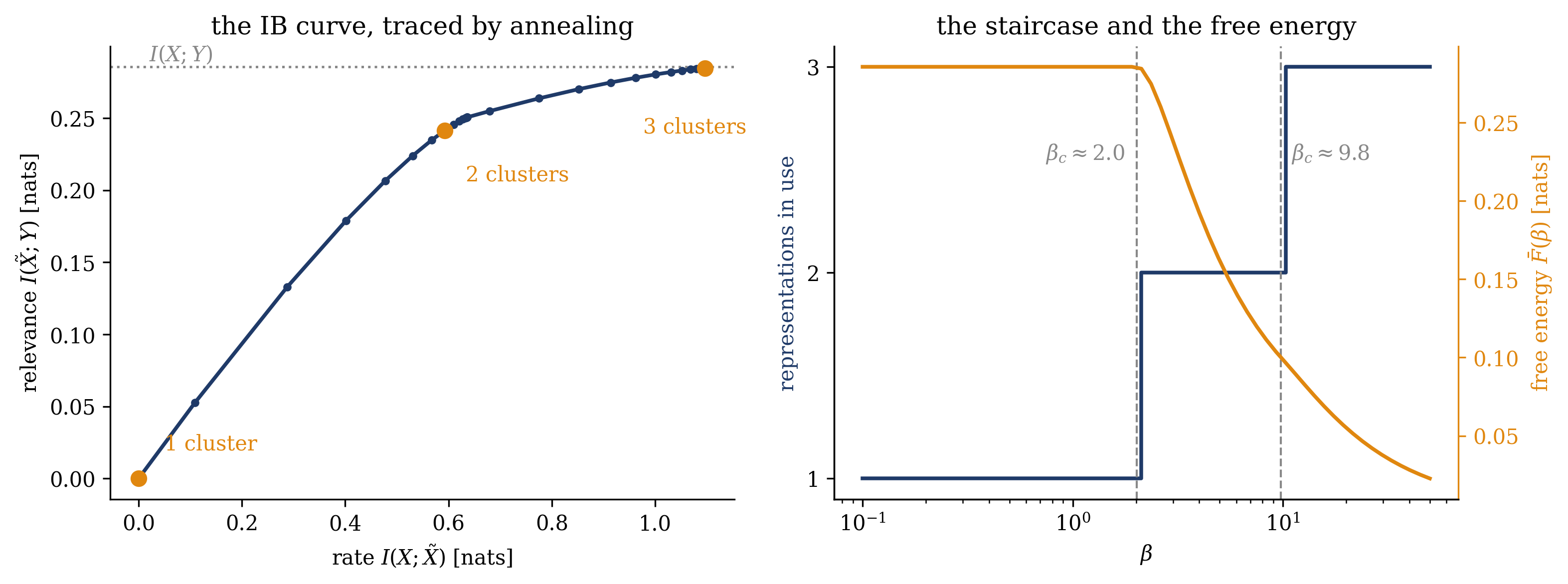
Figure 25.2: The IB curve and its phase transitions, computed exactly by annealed Blahut–Arimoto on the twelve-state toy (\(|\tilde{X}| = 8\), sixty-three values of \(\beta \in [0.1, 50]\), warm-started; fixed seed). Left: the information plane. The optimal encoders trace the concave frontier from the origin to saturation at \(I(X;Y) = 0.286\) nats (dotted); the two-cluster plateau passes through \((0.59, 0.24)\) at \(\beta = 4\), and by \(\beta = 50\) the three-cluster solution reaches \(I(\tilde{X};Y) = 0.285\) nats — \(99.7\%\) of the total — at rate \(I(X;\tilde{X}) = 1.098 \approx \ln 3\). Right: the number of distinct representations in use (navy, left axis) climbs the staircase \(1 \rightarrow 2 \rightarrow 3\) at the critical temperatures \(\beta_c \approx 2.0\) and \(\beta_c \approx 9.8\) (dashed), while the annealed free energy \(\bar{F}(\beta)\) (orange, right axis) descends from exactly \(I(X;Y)\) in the hot limit — where the single decoder is \(p(y)\) and the mean distortion is the whole of the information — toward zero, kinking at each transition.
The left panel of Figure 25.2 is the schematic of Figure 25.1 made quantitative. The frontier rises steeply while relevance is cheap, passes the two-cluster plateau at \((0.59, 0.24)\) — a rate just below the \(\ln 3 - \frac{2}{3}\ln 2 = 0.637\) nats of a hard three-way split’s first stage, buying \(84\%\) of the available relevance — and saturates: at \(\beta = 50\) the three-cluster encoder holds \(I(\tilde{X};Y) = 0.285\) of the \(0.286\) nats available, at a rate of \(\ln 3\). Eight representation slots were on offer and the solution declines five of them; the cap never binds, because the temperature decides. The right panel shows that decision unfold. The number of representations in use climbs \(1 \rightarrow 2 \rightarrow 3\) at \(\beta_c \approx 2.0\) — where the well-separated third group breaks away — and \(\beta_c \approx 9.8\), where the two similar groups finally part; between the transitions the count is rigid while the free energy \(\bar{F}(\beta)\) (orange) glides down, kinking at each split. Its hot end is a check on Equation 25.3 done by hand: with one cluster the decoder is \(p(y)\), the distortion of every input is \(D_\mathrm{KL}[p(y \mid x) \| p(y)]\), and the mean distortion is exactly \(I(X;Y) = 0.286\) nats — the figure’s orange curve starts there to the fourth decimal.
Show code
cmap = LinearSegmentedColormap.from_list("navy", ["#ffffff", NAVY])def merged(q, tol=0.05):# merge slots whose decoders coincide; order columns by their decoder's <y> p_t = p_x @ q p_y_t = (p_xy.T @ q) / (p_t[None, :] + EPS) groups = []for t in np.where(p_t >1e-3)[0]:for g in groups:if np.abs(p_y_t[:, t] - p_y_t[:, g[0]]).max() < tol: g.append(t);breakelse: groups.append([t]) groups.sort(key=lambda g: np.arange(ny) @ p_y_t[:, g[0]])return np.column_stack([q[:, g].sum(axis=1) for g in groups])fig, axes = plt.subplots(1, 3, figsize=(10.6, 3.6))for ax, b_s inzip(axes, [0.5, 4.0, 40.0]): b = betas[np.argmin(np.abs(betas - b_s))] m = merged(snap[b]) ax.imshow(m, cmap=cmap, vmin=0, vmax=1, aspect="auto")for yline in (3.5, 7.5): ax.axhline(yline, color=ORANGE, lw=1.4) ax.set_title(rf"$\beta = {b_s:g}$", fontsize=12) ax.set_xlabel(r"representation $\tilde{x}$") ax.set_xticks(range(m.shape[1])) ax.set_yticks([0, 3, 7, 11], ["1", "4", "8", "12"]) ax.tick_params(length=0)axes[0].set_ylabel(r"input $x$")fig.tight_layout()plt.show()
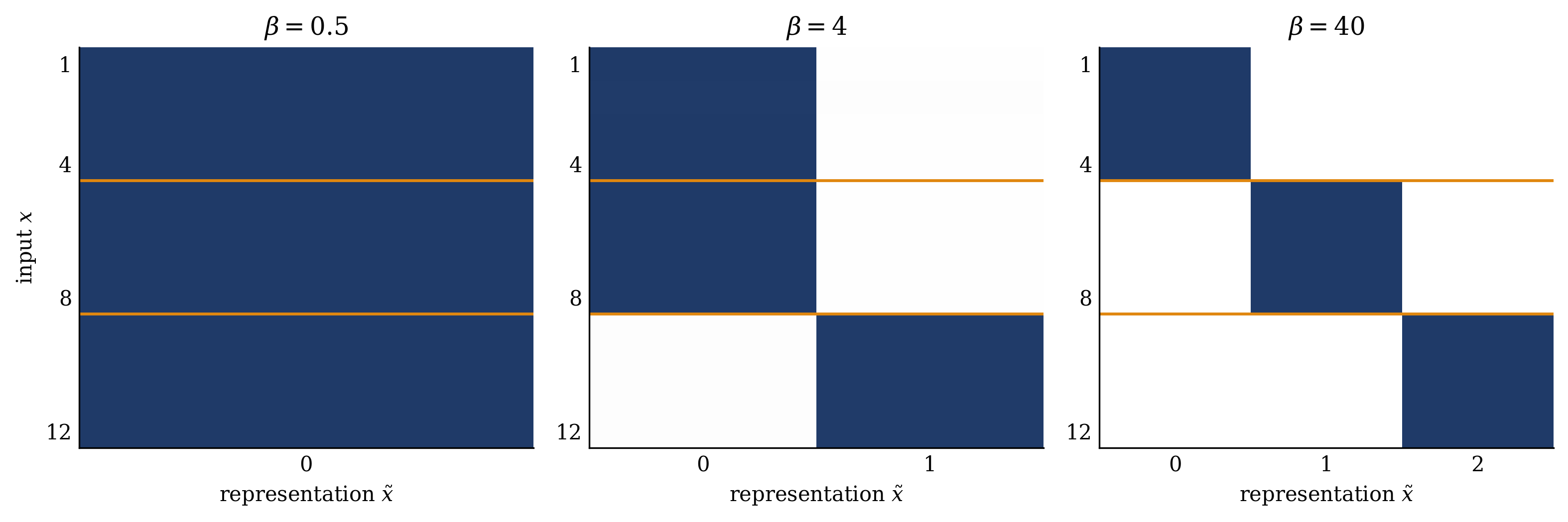
Figure 25.3: The encoder is a Boltzmann distribution sharpening as it cools: the optimal \(p(\tilde{x} \mid x)\) of the same sweep, at \(\beta = 0.5\), \(4\), and \(40\) (left to right; rows are inputs \(x\), columns the representations in use, duplicate slots merged; darker is more probable, orange rules mark the three input groups). Hot, every input relaxes onto the same single description. At \(\beta = 4\), past the first transition, the third group has committed to its own representation while the first two share one, a percent-level leak still crossing the divide. Cold, the assignment is a near-hard three-way partition — the sufficient-statistic limit approached from finite temperature.
Figure 25.3 shows the same physics from inside one conditional. At \(\beta = 0.5\) the encoder matrix is a single uniform column — the Boltzmann distribution at high temperature, flat over its states. At \(\beta = 4\) the first symmetry has broken: inputs \(9\)–\(12\) occupy their own representation, inputs \(1\)–\(8\) share a second, about one percent of each conditional still leaks across the divide, and the two similar groups are not yet distinguished at all. At \(\beta = 40\) the partition is all but hard, three blocks for three groups, and further cooling would only sharpen the edges: within the range plotted, no fourth description condenses, because resolving the \(\pm 0.02\) perturbations that distinguish inputs within a group carries a distortion gain too small to pay for at these temperatures. The tutorial (16–18, Ph12 106) runs this entire construction where the answer is not transparent: an IB curve computed on a real classifier, with \(p(y \mid x)\) a trained network’s output rather than a table, and its reorganizations found by the same annealing.
A representation is the Boltzmann distribution of a rate–distortion free energy — compression traded against relevance at inverse temperature \(\beta\) — so representation learning is the variational free-energy minimization of Weeks 5 and 7, one module later.
25.7 Outlook: from one system’s transitions to inference at large
The warm-up card covers a hand calculation: the IB Lagrangian for a two-symbol source, minimized to the point where the coupled dependence forces iteration — Tishby, Pereira, and Bialek (1999) §2–3 read against the derivation of Section 25.3.
That lecture generalizes today’s most physical observation. The bottleneck’s staircase — a representation reorganizing discontinuously at critical values of a control parameter — is not a curiosity of this toy but the signature of a broad and quantitative theory: inference problems at large undergo phase transitions. Detecting communities in a network, recovering a planted low-rank signal in a noisy matrix, learning a rule from examples — each has sharp thresholds in signal strength or data volume separating an impossible phase, where no method can succeed, from a recoverable one, and often a further threshold separating what is information-theoretically possible from what any known efficient algorithm achieves. The tools are this course’s: partition functions over hypotheses, free energies whose competing minima are “signal found” and “signal lost,” and message-passing algorithms (Section 12.3) whose fixed points delimit the algorithmic phase (Zdeborová and Krzakala 2016). The next lecture derives the flagship example and closes with the outlook onto the field’s current frontier.
Week 14 then ends the course: Lecture 1 reads every module off a single free-energy functional — the synthesis this week prepares — and the next lecture is review and exam preparation. From the Boltzmann distribution of Week 1 to the encoder of Week 13, one variational principle has recurred with different constraints attached, and the last constraint — an information budget — turned it into a theory of representation.
Alemi, Alexander A., Ian Fischer, Joshua V. Dillon, and Kevin Murphy. 2017. “Deep Variational Information Bottleneck.” In ICLR 2017.
Dayan, Peter, Geoffrey E. Hinton, Radford M. Neal, and Richard S. Zemel. 1995. “The Helmholtz Machine.”Neural Computation 7 (5): 889–904. https://doi.org/10.1162/neco.1995.7.5.889.
Friston, Karl J. 2010. “The Free-Energy Principle: A Unified Brain Theory?”Nature Reviews Neuroscience 11 (2): 127–38. https://doi.org/10.1038/nrn2787.
Higgins, Irina, Loic Matthey, Arka Pal, Christopher Burgess, Xavier Glorot, Matthew Botvinick, Shakir Mohamed, and Alexander Lerchner. 2017. “\(\beta\)-VAE: Learning Basic Visual Concepts with a Constrained Variational Framework.” In International Conference on Learning Representations (ICLR).
Rose, Kenneth. 1998. “Deterministic Annealing for Clustering, Compression, Classification, Regression, and Related Optimization Problems.”Proceedings of the IEEE 86 (11): 2210–39. https://doi.org/10.1109/5.726788.
Saxe, Andrew M., Yamini Bansal, Joel Dapello, Madhu Advani, Artemy Kolchinsky, Brendan D. Tracey, and David D. Cox. 2018. “On the Information Bottleneck Theory of Deep Learning.” In International Conference on Learning Representations (ICLR). https://doi.org/10.1088/1742-5468/ab3985.
Shwartz-Ziv, Ravid, and Naftali Tishby. 2017. “Opening the Black Box of Deep Neural Networks via Information.”
Tishby, Naftali, Fernando C. Pereira, and William Bialek. 1999. “The Information Bottleneck Method.” In Proc. 37th Allerton Conference on Communication, Control, and Computing, 368–77.
Tishby, Naftali, and Noga Zaslavsky. 2015. “Deep Learning and the Information Bottleneck Principle.” In 2015 IEEE Information Theory Workshop (ITW), 1–5. https://doi.org/10.1109/ITW.2015.7133169.
Zdeborová, Lenka, and Florent Krzakala. 2016. “Statistical Physics of Inference: Thresholds and Algorithms.”Advances in Physics 65 (5): 453–552. https://doi.org/10.1080/00018732.2016.1211393.